Categories
Research

Reconstruction of Implicit Non-Manifold Surfaces

I. Introduction

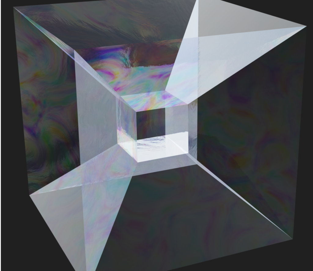
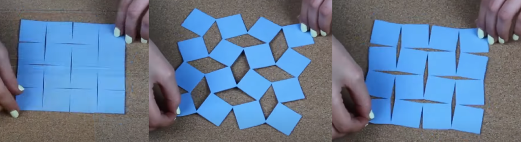
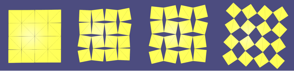
The majority of surfaces in our daily lives are manifold surfaces. Roughly speaking, a manifold surface is one where, if you zoom in close enough at every point, the surface begins to resemble a plane. Most algorithms in computer graphics and digital geometry have historically been tailored for manifold surfaces and fail to preserve or even process non-manifold structures. Non-manifold geometries appear naturally in many settings however. For instance, a dress shirt pocket is sewn onto a sheet of underlying fabric, and these seams are fundamentally non-manifold. Non-manifold surfaces arise in nature in a variety of other settings too, from dislocations in cubic crystals on a molecular level, to the tesseract structures that appear in real world soap films (see Figure 1) [Ishida et al. 2020, Ishida et al. 2017].

Figure 1: Soap film covering the non-manifold minimal surface of a tesseract structure.

The study of soap films connects very closely to a rich vein of study concerning the geometry of minimal surfaces with boundary. The explicit representation of minimal surfaces has a rich history in geometry processing, dating back to the classic paper by Pinkall and Polthier 1993 . Since then, there has been continued study within computer graphics for robust algorithms for computing minimal surfaces, something which is broadly referred to as “Plateau’s Problem”.

Recent work in computer graphics [Wang and Chern 2021] introduced the idea of computing minimal surfaces by solving an “Eulerian” style optimization problem, which they discretize on a grid. In this SGI project, we explored an extension of this idea to the non-manifold setting.

II. Surface Representations

There are multiple ways to digitally represent surfaces, each one with different properties, advantages and disadvantages. Explicit surface representations, such as surface meshes, are easy to model and edit in an intuitive way by artists, but are not very convenient in other settings like constructive solid geometry (CSG). In contrast, implicit surfaces allow to perform morphological operations, and recent advances, such as neural implicits, are also exciting and promising [Xie et al. 2022].

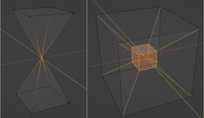
One practical advantage of explicit surface representations like triangle meshes is that they are flexible and intuitive to work with. Triangle meshes are a very natural way to represent manifold surfaces, i.e. surfaces that satisfy the property that the neighborhood of every point is locally similar to the Euclidean plane (or half-plane, in the case of boundaries), and many applications, like 3D printing, require target geometries to be manifold. Triangle meshes can naturally capture non-manifold features as well by including vertices that connect otherwise disjoint triangle fans as in (Figure 2, left) or by edges that are shared by more than two faces (Figure 2, right).

Figure 2: Examples of non-manifold meshes. Non-manifold vertices and edges are highlighted in orange. Left: mesh containing a non-manifold vertex. Right: mesh containing non-manifold edges. Blender highlights faces composed solely by non-manifold edges.

However, in many real world settings, geometric data is not naturally acquired as or represented by a triangle mesh. In applications ranging from medical imaging to constructive solid geometry, the preferred geometric representation is as implicit surfaces.

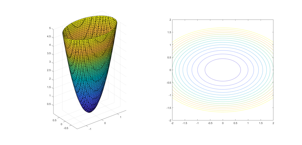
In 2D, implicit surfaces can be described by a function \(f: \mathbb{R}^{2} \rightarrow \mathbb{R}\) that is described by the points \((x, y) \in \mathbb{R}^{2}\) such that \(f(x, y) = c\) for some real value \(c\). By varying the values of \(c\) a set of curves, called level sets, can be used to represent the surface. Figure 3 shows two representations of the same paraboloid, one using an explicit triangle mesh representation (left) and one using level sets of the implicit function (right).

Figure 3: Two distinct representations of the same surface. Left: explicit representation of a hyperboloid using a surface mesh. Right: implicit representation of a hyperboloid using level sets.

While non-manifold features are naturally represented in explicit surface representations, one limitation of implicit surfaces and level sets is that they do not naturally admit a way to represent geometries with non-manifold topology and self-intersections. In this project we focused on studying a way of representing implicit surfaces based on the mathematical machinery of integrable vector fields defined on a background domain.

III. Representing Implicit Surfaces as Integrable Vector Fields

In this project our goal was to explore implicit representations of non-manifold surfaces. To do this, we set out to represent implicit function implicitly, as an integrable vector field.

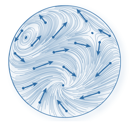
A vector field \(V: \mathbb{R}^{m} \rightarrow \mathbb{R}^{n}\) is a function that corresponds a vector for each point in space. In our case, we are interested in cases where \(m = n = 2\) or \(m = n = 3\); see Figure 4 for an illustration of a vector field defined on a surface.
Vector field design and processing is a vast topic, with enough content to fill entire courses on the subject – we refer the interested reader to Goes et al. 2016 and Vaxman et al. 2016 for details.

Figure 4: Vector field defined on a surface. Source: Goes et al. 2016.

One way of thinking of implicit surfaces is as constant valued level sets of some scalar function defined over the entire domain. Our approach was to represent this scalar function as a function of a vector field which we received as an input to our algorithm.

To reconstruct a scalar field from the vector field, it is necessary to integrate the field, which led us into the discussion of integrability of vector fields. A vector field is integrable when it is the gradient of a scalar function. More precisely, the vector field \(V\) is integrable if there is a scalar function \(f\) such that \(V = \nabla f\).

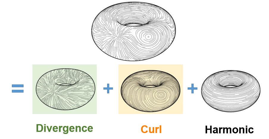
Since it can be arbitrarily hard to find the function \(f\) such that \(V = \nabla f\), or this function may even not exist at all, an equivalent but more convenient condition to check if a vector field is integrable is whether the vector field it is curl-free, that is, if \(\nabla \times V = 0\) for all points in space (Knöppel et al. 2015, Polthier and Preuß 2003). If the vector field is not curl-free, then it is non-integrable, and there is no \(f\) such that \(V = \nabla f\). A possible approach to remove non-integrable features is to apply the Helmholtz-Hodge decomposition, which decomposes the field \(V\) into the sum of three distinct vector fields:

\(\begin{equation} V = F + G + H \end{equation}\)

such that \(F\) is curl-free, \(G\) is divergence-free and \(H\) is a harmonic component. The curl-free \(F\) component is integrable. Figure 5 visualizes this decomposition.

Figure 5: Helmholtz-Hodge decomposition of a vector field defined over a surface. Source: Adapted from Goes et al. 2016.

The non-integrable regions of the vector field correspond to regions where the vector field vanishes or is undefined, also called singularities. For a standard vector field, singular points can be located by checking if the Jacobian is a singular matrix. For implicit non-manifold surfaces, removing the singularities using Helmholtz-Hodge decomposition is not particularly interesting, because the singularities are the cause of the non-manifold features that we want to preserve. At the same time, the singularities prevent the integration of the field, which we wanted to do to reconstruct the levels sets of the implicit function. This dichotomy suggests two different approaches to reconstructing the surface, as described in Section V.

IV. Representing Non-Manifold surfaces as Integrable Frame Fields

Frame Fields or poly-vector fields are generalizations of vector fields which store multiple distinct directions at each point. This terminology was introduced to the graphics literature by Panozzo et. al. 2014, and a technique for generating such integrable fields was presented by Diamanti et. al. 2015.

Animation 1 illustrates one curious phenomenon related to the topology of directional and frame fields. Assume each direction is uniquely labelled (e.g., each different direction is assigned a different color). If you start labelling an arbitrary direction and smoothly circulates around the singularity, trying to consistently label each direction with a unique color, this necessarily causes a mismatch between the initial label and the final label at the starting point. As can be seen in the last frame of the animation, a flow line that was initially assigned a green color was assigned a different color (red) in the last step, characterizing a mismatch between the initial and final label of that flow line. This happens for all the directions.

Animation 1: Failure to uniquely label each flow line direction around a singularity in a directional field. The initial flow line was labelled green. Source: Adapted from Knöppel et al. 2013.

V. Surface Reconstruction

The task can be specifically described as follows: given a frame field defined on a volumetric domain (i.e., a tetrahedral mesh), our goal is to reconstruct a non-manifold surface mesh that represents a non-manifold implicit surface. Two distinct approaches were explored: (i) stream surface tracing based on the alignment of the vector fields and (ii) Poisson surface reconstruction.

V.1. Stream Surface Tracing

The first approach consisted in using stream surfaces to represent the non-manifold surface. Stream surfaces are surfaces whose normal are aligned with one of the three vectors of the frame field. These types of surfaces are usually employed to visualize flows in computational fluid dynamics (Peikert and Sadlo 2009). Many ideas of the algorithm we explored are inspired by Stutz et al. 2022, which further extends the stream surface extraction with an optimization objective to generate multi-laminar structures for topology optimization tasks.

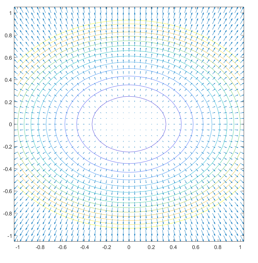
It is known that the gradient \(\nabla f\) of a function \(f\) is perpendicular to the level sets of the function (see Figure 6 for a visual demonstration). Therefore, if we had the gradient of the function, it would be possible to extract a surface by constructing a triangle mesh whose normal vectors of each face are given by the gradient of the function. The main idea of the stream surface tracing is that the input frame field can be used as an approximation of the gradient of the function that we are trying to reconstruct. In other words, the normal vector of the surface is aligned with one of the vectors of the frame field.

Figure 6: the gradient \(\nabla f\) of a function \(f\) is perpendicular to the level sets of \(f\).

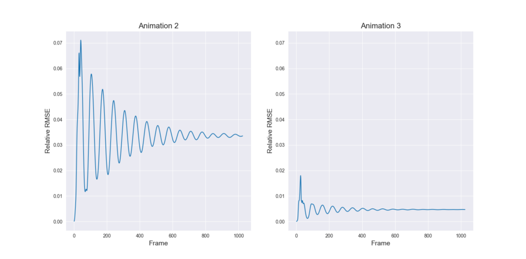
Animation 2 displays a step-by-step sequence for the first two tetrahedrons that are visited by the stream surface tracing algorithm, that proceeds as follows:

  1. Choose an initial tetrahedron to start the tracing;
  2. Compute the centroid of the first tetrahedron;
  3. Choose one of the (three) vectors of the frame field as a representative of the normal vector of the surface;
  4. Intersect a plane with the centroid of the tetrahedron such that the previous chosen vector is normal to this plane;
  5. Choose a neighbor tetrahedron that shares a face with the edges that were intersected in the previous step;
  6. For the new tetrahedron, compute the centroid and choose a vector of the frame field (similar to steps 2 and 3);
  7. Project the midpoint of the edge of the previous plane into a line that passes through the centroid of the new tetrahedron.
  8. Intersect a plane with the point computed in the previous step and the new tetrahedron.
  9. Repeat steps 5 through 8 until all tetrahedrons are visited.

After repeating the procedure for all the tetrahedrons in the volumetric domain, a stream surface is extracted that tries to preserve non-manifold features.

Animation 2: Illustration of the main steps of the stream surface algorithm applied to the first two tetrahedra. This procedure is repeated for all tetrahedra in the volumetric domain.
V.1.1 – Results using Vector Fields

Animation 3 demonstrates the stream surface tracing algorithm for a frame field defined on a volumetric domain. In this case, it can be seen that the algorithm extracts a Möbius strip, which is a non-orientable manifold surface.

Animation 3: Stream surface tracing incrementally reconstructing a Möbius strip.

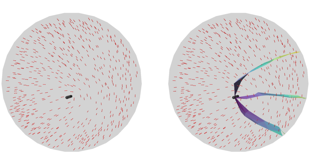
However, the Möbius strip is still a manifold surface and we want to reconstruct non-manifold surfaces. As an example of a surface with non-manifold structures, consider Figure 7. Figure 7, left, shows a frame field and the singularity graph associated with it, while Figure 7, right, presents the surface by the algorithm. The output of the algorithm is a surface mesh containing a non-manifold vertex in the neighborhood of the singular curve, indicating the non-integrability of the field.

Figure 7: Left: frame field and associated singular curve. Right: surface extracted using the surface tracing algorithm. Notice the formation of a T-junction in the neighborhood of the singular curve.

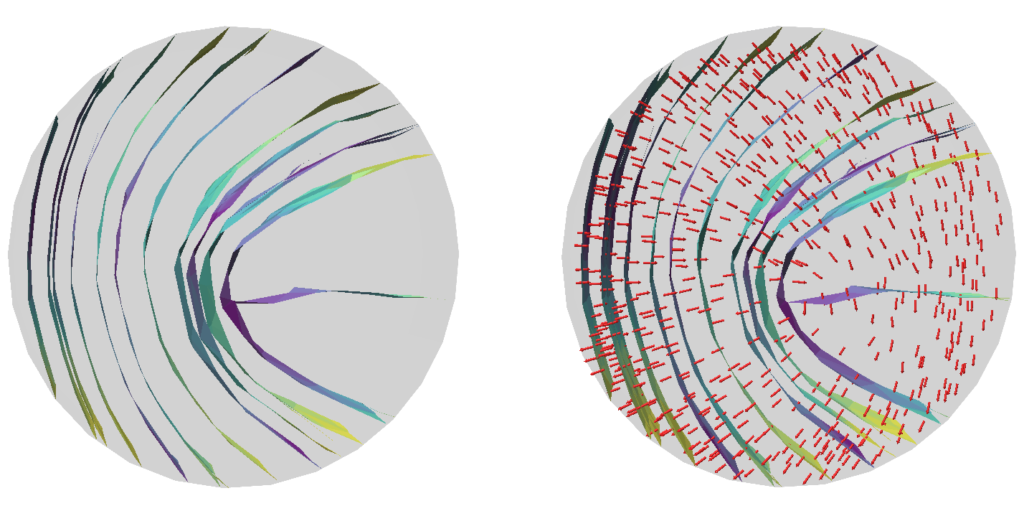
By applying the stream surface tracing algorithm starting from different tetrahedrons, it is possible to trace multiple level sets of the implicit non-manifold surface. Figure 8 displays the result of such procedure, where multiple strips were extracted corresponding to different level sets. Figure 8, right, shows the frame field together with the extracted surfaces: here, it is possible to notice that each vector is approximately normal to the surfaces. This was expected, since the assumption of the algorithm was that the frame field can be used as an approximation of the gradient of the function we want to reconstruct.

Figure 8: Left: reconstructed surfaces for different level sets of the function. Right: surfaces and the corresponding vector field. Notice how the vectors are roughly orthogonal to the level sets, as expected.
V.1.2. Volumetric Frame Fields: Working with Frame Fields in 3D volumes

Implicit functions, as described above, are real-valued functions with infinitely many values. To represent them on a computer, some sort of spatial discretization is necessary. Two common choices are to discretize the space using regular grids or unstructured meshes where each element is a triangle or a tetrahedron. This discretization corresponds to an Eulerian approach: for a fixed discretized domain, the values of the vector fields associated with the implicit functions are observed in fixed locations in space. In this project, tetrahedral meshes are used to discretize the space and fill the volume where the functions are defined.

A tetrahedral mesh is similar to a triangle mesh, but augmented with additional data for each tetrahedron. Formally, a tetrahedral mesh \(\mathcal{M}\) is defined by a set \({\mathcal{V}, \mathcal{E}, \mathcal{F}, \mathcal{T}}\) of vertices, edges, faces and tetrahedrons, respectively. Each tetrahedron is composed of 4 vertices, 6 edges and 4 faces. The edges and faces of one tetrahedron may be shared with adjacent tetrahedrons, which allow to traverse the mesh. More importantly, this allows to define the vector field using the tetrahedral mesh as a background domain to discretize the function over this volumetric space.

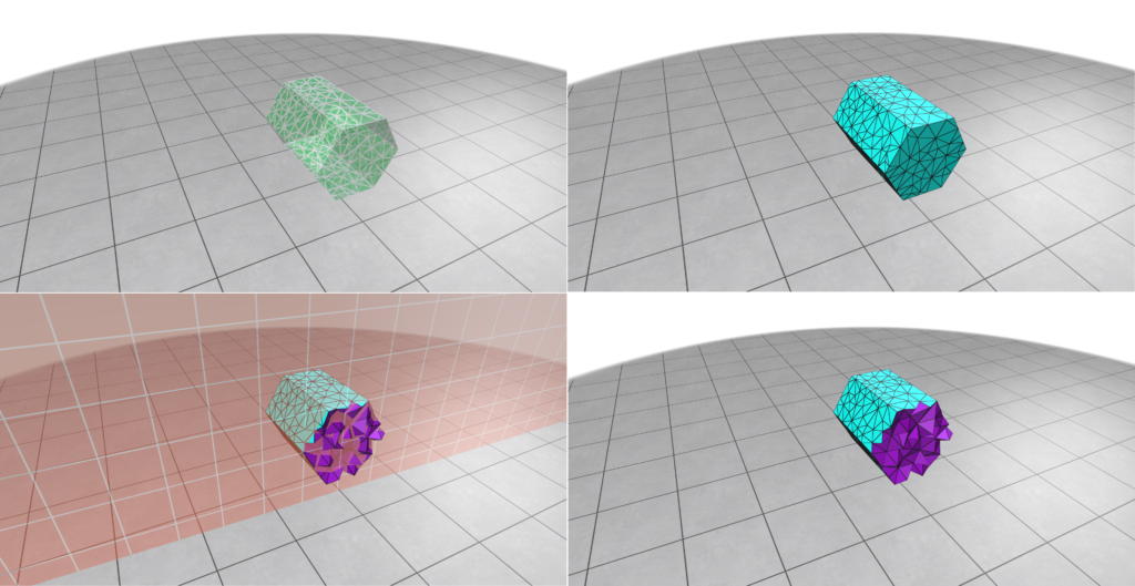
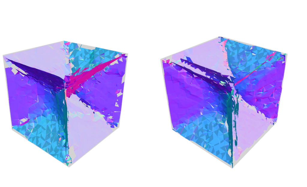
As input, we start with a boundary mesh enclosing a volume (Figure 9, top left). Bear in mind that this boundary mesh does not fill the space, but only specifies the boundary of a region of interest. We can fill the volume using a tetrahedral mesh (Figure 9, top right). This tetrahedralization can be done using Fast Tetrahedral Meshing in the Wild, for instance. It is important to notice that, in contrast to a surface polygon mesh, a tetrahedral mesh is a volume mesh in the sense that it fills the volume enclosed by it. If we slice the tetrahedral mesh with a plane (Figure 9, bottom left and bottom right), we can see that the interior of the tetrahedral mesh is not empty (as would be the case for a surface mesh) and that the interior volume is fully filled. In Figure 9, the interior faces of the tetrahedrons were colored in purple while the boundary faces were colored in cyan.

Figure 9: Tetrahedralization of a boundary domain. Starting with a boundary domain bounded by a surface mesh (top left), the domain is discretized using tetrahedrons (top right). Unlike a surface mesh, a volumetric mesh fills the interior space of the volume it discretizes (bottom row).

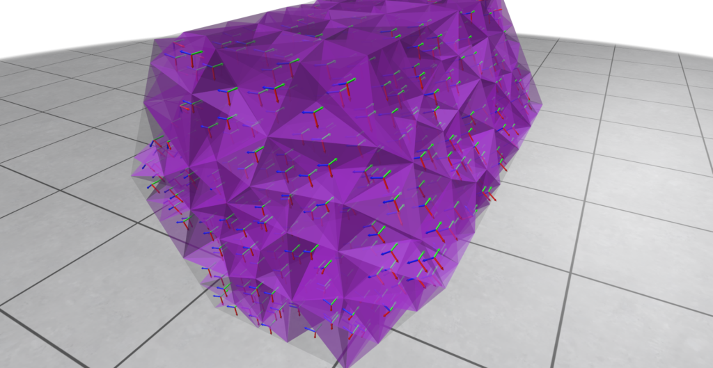
Three distinct vector fields \(U, V, W\) constitute a volumetric frame field if they form an orthonormal basis at each point in space. As mentioned, we work with frame fields defined on a volumetric domain as a representation of the implicit non-manifold surface. Each tetrahedron will be associated with three orthogonal vectors, as shown in Figure 10.

Figure 10: Sample of data used to represent a non-manifold implicit surface. The domain was discretized using tetrahedral meshes (purple). Each tetrahedron is associated with three orthogonal vectors, that constitute a volumetric frame field.

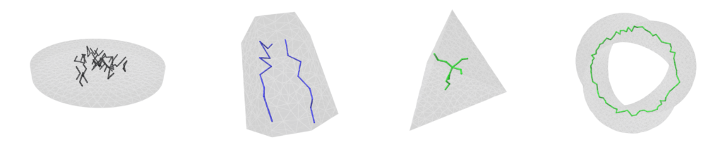
The previous idea of labelling directions around a point can be useful to detect singularities in our frame fields. The same idea can be extended to volumetric frame fields, where singularities create singular curves on the volumetric domain. These curves are denominated as singularity graphs. Figure 11 shows the singularity graphs for some frame fields. See Nieser et al. 2011 for details. Identifying the singular curves on the frame fields is equivalent to identifying its non-integrable regions.

Figure 11: Singularity graphs of the volumetric frame fields.
V.1.3. Results using Volumetric Frame Fields

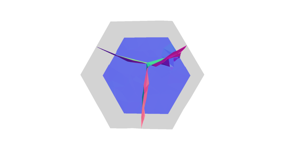
Another example is provided in Figure 12, where the volumetric frame field is defined on a hexagonal boundary mesh. The output presents a non-manifold junction through a non-manifold vertex.

Figure 12: reconstructed surface for a hexagonal boundary mesh.

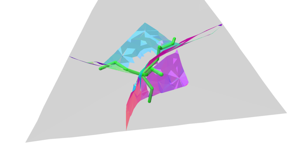
As a harder test case, it can be seen in Figure 13 that the resulting surface extracted by the algorithm is not a perfectly closed mesh. While the surface tries to follow the singularity graph (in green), it fails to self-intersect in some regions, creating undesirable gaps.

Figure 13: reconstructed surface for a tetrahedral boundary mesh and the singularity graph (in green) associated with the volumetric frame field. The surface has an overall structure that resembles the junction present in the singularity graph, but in this case the algorithm wasn’t able to extract a mesh without holes.

Finally, we tested the algorithm to reconstruct the non-manifold minimal tesseract, presented in Figure 1. Two points of view of the output are presented in Figure 14. While the traced mesh has a structure similar to the desired surface, the result could still be further improved. The mesh presents cracks in the surface and some almost disconnected regions. We applied hole filling algorithms, such as those provided by MeshLab, as an attempt to fix the issue, but they weren’t capable of closing the holes for any combination of parameters tested.

Figure 14: reconstructed surface for the non-manifold minimal surface tesseract. The reconstruction preserves the overall structure of the desired surface. However, the algorithm fails to create a surface without holes and produces some regions that are mostly disconnected from the surface.

V.2. Poisson Surface Reconstruction

The second approach consisted in investigating the classic Poisson Surface Reconstruction algorithm by Kazhdan et al. 2006 for our task. Specifically, our goal was to evaluate whether the non-manifold features were preserved using this approach and, if not, where exactly it fails.

Given a differentiable implicit function \(f\), we can compute its gradient vector field \(G = \nabla f\). This can be done either analytically, if there is a closed-formula for \(f\), or computationally, using finite-element methods or discrete exterior calculus. Conversely, given a gradient vector field \(G\), we can integrate \(G\) to compute the implicit function \(f\) that generates the starting vector field.

Note that since it was assumed that \(G\) is a gradient vector field, and not an arbitrary vector field, this means that \(G\) is integrable. If this is the case, we know that a function \(f\) whose gradient vector field is \(G\) exists; we just need to find it. However, in practice, the input of the algorithm may be a vector field \(V\) which is not exactly integrable due to noise or sampling artifacts. How can \(f\) be computed in all these cases?

One core idea of the Poisson Surface Reconstruction algorithm consists in reconstructing \(f\) using a least-squares optimization formulation:

\(\begin{equation} \tilde{f} = \arg \min_{f} \left |V – \nabla f \right |^{2} \end{equation}\)

For a perfectly integrable vector field (i.e., a gradient vector field), it would theoretically be possible to compute \(\tilde{f} = f\) such that \(\nabla \tilde{f} = V\) and reconstruct \(f\) exactly. The advantage of this formulation is that even in cases where the vector field \(V\) is not exactly integrable, it will reconstruct the best approximation of \(f\) by minimizing the least-squares error.

In the case of our frame fields representing non-manifold surfaces, the existence of singularities in the field means that it will necessarily be non-integrable. It is expected that the equality \(\nabla \tilde{f} = V\) fails precisely in the regions containing singular points, but we wanted to evaluate the performance of a classic algorithm on our data.

V.2.1 – Results using Volumetric Frame Fields

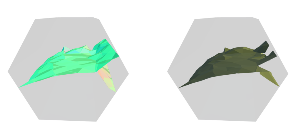
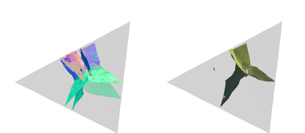
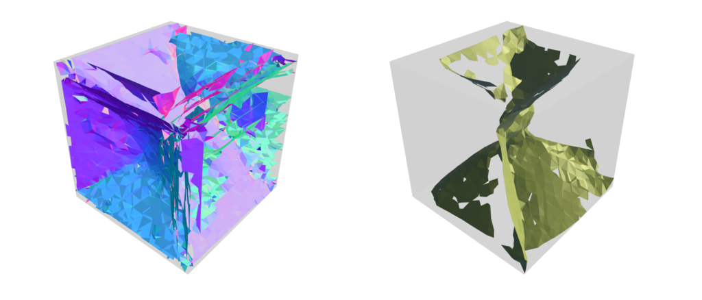
Figure 15 and Figure 16 present comparisons between the surface extracted by Stream Surface Tracing and Poisson Surface Reconstruction algorithm for two different inputs. While for the hexagonal boundary mesh (Figure 15) both algorithms have a similar output, for the tetrahedral boundary mesh (Figure 16) Poisson Surface Reconstruction generates a surface closer to the desired non-manifold junction.

Figure 15: Comparison between the Stream Surface Tracing algorithm (left) and the Poisson Surface Reconstruction (right) for the volumetric frame field with hexagonal boundary mesh.
Figure 16: Comparison between the Stream Surface Tracing algorithm (left) and the Poisson Surface Reconstruction (right) for the volumetric frame field with tetrahedral boundary mesh. In this case, Poisson Surface Reconstruction extracts a surface that is closer to the desired junction in comparison to the Stream Surface Tracing.

Remarkably, the Poisson Surface Reconstruction fails badly for the non-manifold tesseract, as shown in Figure 17. While the Stream Surface Tracing doesn’t extract a perfect surface reconstruction (Figure 17, left), it is much closer to the tesseract than the surface reconstructed by the Poisson Surface Reconstruction (Figure 17, right).

Figure 17: Comparison between the Stream Surface Tracing algorithm (left) and the Poisson Surface Reconstruction (right) for the volumetric frame field defined for the tesseract structure. In this case, Poisson Surface Reconstruction drastically fails to preserve the non-manifold structure of the target surface.

VI. Conclusions and Future Work

In this project we explored multiple surface reconstruction algorithms that could possibly preserve non-manifold structures from frame fields defined on tetrahedral domains. While the algorithms could extract surfaces that present the overall structure desired, for many inputs the mesh displayed artifacts such as cracks or components that aren’t completely connected, such as non-manifold vertices where a non-manifold edge was expected. As future work, we consider using the singularity graph to guide the tracing as an attempt to close the holes in the mesh. Another possible direction would be to explore the usage of the singularity graph in the optimization process used in the Poisson Surface Reconstruction algorithm.

I would like to thank Josh Vekhter, Nicole Feng and Marco Ravelo for the mentoring and patience to guide me through the rich and beautiful theory of frame fields. Furthermore, I would like to thank Justin Solomon for the hard work on organizing SGI and baking beautiful singular pies.

VII. References

Ishida, Sadashige, et al. “A model for soap film dynamics with evolving thickness.” ACM Transactions on Graphics (TOG) 39.4 (2020): 31-1.

Ishida, Sadashige, et al. “A hyperbolic geometric flow for evolving films and foams.” ACM Transactions on Graphics (TOG) 36.6 (2017): 1-11.

Pinkall, Ulrich, and Konrad Polthier. “Computing discrete minimal surfaces and their conjugates.” Experimental mathematics 2.1 (1993): 15-36.

Wang, Stephanie, and Albert Chern. “Computing minimal surfaces with differential forms.” ACM Transactions on Graphics (TOG) 40.4 (2021): 1-14.

Xie, Yiheng, et al. “Neural fields in visual computing and beyond.” Computer Graphics Forum. Vol. 41. No. 2. 2022.

De Goes, Fernando, Mathieu Desbrun, and Yiying Tong. “Vector field processing on triangle meshes.” ACM SIGGRAPH 2016 Courses. 2016. 1-49.

Vaxman, Amir, et al. “Directional field synthesis, design, and processing.” Computer graphics forum. Vol. 35. No. 2. 2016.

Knöppel, Felix, et al. “Stripe patterns on surfaces.” ACM Transactions on Graphics (TOG) 34.4 (2015): 1-11.

Polthier, Konrad, and Eike Preuß. “Identifying vector field singularities using a discrete Hodge decomposition.” Visualization and mathematics III. Springer Berlin Heidelberg, 2003.

Panozzo, Daniele, et al. “Frame fields: Anisotropic and non-orthogonal cross fields additional material.” Proceedings of the ACM TRANSACTIONS ON GRAPHICS (PROCEEDINGS OF ACM SIGGRAPH (2014).

Diamanti, Olga, et al. “Integrable polyvector fields.” ACM Transactions on Graphics (TOG) 34.4 (2015): 1-12.

Knöppel, Felix, et al. “Globally optimal direction fields.” ACM Transactions on Graphics (ToG) 32.4 (2013): 1-10.

Peikert, Ronald, and Filip Sadlo. “Topologically relevant stream surfaces for flow visualization.” Proceedings of the 25th Spring Conference on Computer Graphics. 2009.

Stutz, Florian Cyril, et al. “Synthesis of frame field-aligned multi-laminar structures.” ACM Transactions on Graphics (TOG) 41.5 (2022): 1-20.

Hu, Yixin, et al. “Fast tetrahedral meshing in the wild.” ACM Transactions on Graphics (TOG) 39.4 (2020): 117-1.

Nieser, Matthias, Ulrich Reitebuch, and Konrad Polthier. “Cubecover–parameterization of 3d volumes.” Computer graphics forum. Vol. 30. No. 5. Oxford, UK: Blackwell Publishing Ltd, 2011.

Kazhdan, Michael, Matthew Bolitho, and Hugues Hoppe. “Poisson surface reconstruction.” Proceedings of the fourth Eurographics symposium on Geometry processing. Vol. 7. 2006.

Categories
Research

Multigrid Solver for Curved Surfaces

Video 1: Numerical solution of the heat equation on curved meshes using a geometric multigrid solver.

By SGI Fellows:  Anna Cole, Francisco Unai Caja López, Matheus da Silva Araujo, Hossam Mohamed Saeed

Mentor: Paul Kry

Volunteers: Leticia Mattos Da Silva and Erik Amézquita

I. Introduction

This technical report describes a follow-up to our previous post. One of the original goals of the project was to apply successive self-parameterization to solve differential equations on curved surfaces leveraging a multigrid solver based on Liu et al. 2021. This post reports the results obtained throughout the summer to achieve this objective and wraps-up the project. Video 1 shows an animation of heat diffusion, obtained by solving the heat equation on surface meshes using the geometric multigrid solver.

II. Partial Differential Equations

Partial differential equations (PDEs) are equations that relate multiple independent variables and their partial derivatives. In graphics and animation applications, PDEs usually involve time derivatives and spatial derivatives, e.g., the motion of an object in 3D space through time described by a function \(f(x, y, z, t)\). Frequently, a set of relationships between partial derivatives of a function is given and the goal is to find functions \(f\) satisfying these relationships.

To more easily study and analyze these equations, it is possible to classify them according to the physical phenomena they describe, which are briefly summarized below. Solomon 2015 and Heath 2018 provide extensive details on partial differential equations for those interested in more in-depth discussions on the topic.

Elliptic PDEs are PDEs that describe systems that have already reached an equilibrium (or steady) state. One example of elliptic PDE is the Laplace equation, given by \(\bigtriangleup \mathbf{u} = \mathbf{0}\). Intuitively, starting with values known only at the boundary of the domain (i.e., the boundary conditions), this equation finds a function \(\mathbf{u}\) such that the values in the interior of the domain smoothly interpolate the boundary values. Figure 1 illustrates this description.

Figure 1: Given boundary conditions, the Laplace Equation is satisfied by a function that smoothly interpolates it to the interior.

Parabolic PDEs are equations that describe systems that are evolving towards an equilibrium state, usually related to dissipative physical behaviour. The canonical example of a parabolic PDE is the heat equation, defined as \(\frac{\mathrm{d}}{\mathrm{dt}} \mathbf{u} = \bigtriangleup \mathbf{u}\). The function \(\mathbf{u}\) describes how heat flows with time over the domain, given an initial heat distribution that describes the boundary conditions. This behaviour can be visualized in Animation 1.

Animation 1: Given an initial heat distribution, the heat equation describes how heat flows over the surface as time progresses, until a steady state is reached.

Finally, hyperbolic PDEs describe conservative systems that are not evolving towards an equilibrium state. The wave equation, described by \(\frac{\mathrm{d}^2}{\mathrm{dt^{2}}} \mathbf{u} = \bigtriangleup \mathbf{u}\), is the typical example of a hyperbolic PDE. In this case, the function \(\mathbf{u}\) characterizes the motion of waves across elastic materials or the motion of waves across the surface of water. Animation 2 provides a visual illustration of this phenomenon. One striking difference between the wave equation and the heat equation is that for the former it is not enough to specify initial conditions for \(\mathbf{u}\) at time \(t = 0\); it is also necessary to define initial conditions for the derivatives \(\mathbf{\frac{\mathrm{d}}{\mathbf{dt}} \mathbf{u}}\) at time \(t = 0\).

Animation 2: Given initial boundary conditions for both the function and its first derivative, the wave equation describes the propagation of a wave through time.

In this project, we restricted the implementation to solving the heat diffusion equations on curved triangle meshes (see Crane et al. 2013). This leads to the following time discretization using a backward Euler step:

\(\begin{equation} \frac{\mathrm{d}}{\mathrm{dt}} \mathbf{u} = \bigtriangleup \mathbf{u} \rightarrow (\mathbf{I} – t\mathbf{L}) \mathbf{u}_{t} = \mathbf{u}_{0} \end{equation}\)

where \(\mathbf{u}_{0}\) is the initial heat distribution and \(\mathbf{L}\) is the Laplacian.

To spatially discretize the equation, we used the cotan-Laplacian \(\mathbf{L}\) discretized at a vertex \(i\):

\(\begin{equation} (\mathbf{L}u){i} = \frac{1}{2 A_{i}} \sum_{j \in \mathcal{N}_{i}} \left(\cot \alpha_{ij} + \cot \beta_{ij} \right) \left(u_{j} – u_{i} \right) \end{equation}\)

where \(A_{i}\) is one-third of the sum of the areas of all the triangles incident to vertex \(i\), \(\mathcal{N}_{i}\) denotes the set of adjacent vertices, and \(\alpha_{ij}, \beta_{ij}\) are the angles that oppose the edge \(e_{ij}\) connecting vertex \(i\) to its neighbor \(j\). The result is a linear system \(\mathbf{A}\mathbf{x} = \mathbf{b}\), where \(\mathbf{A} = \mathbf{I} – t\mathbf{L}\) and \(\mathbf{b} = \mathbf{u}_{0}\). This linear system can be solved numerically.

III. Multigrid Method

There is a large variety of methods to numerically solve PDEs. After choosing time and spatial discretization, the PDE may be solved as a linear system. To that end, it is possible to apply a direct solver (e.g., LU decomposition or Cholesky factorization) to find the solution. These methods are exact in the sense that they provide an exact solution in a finite number of steps. One disadvantage of direct solvers approach is that it may be too expensive to frequently recompute the matrix decomposition in cases where the system of equations requires updates. Iterative methods (e.g., Gauss-Seidel and Jacobi) provide an efficient alternative, but at the cost of providing only approximate solutions and having poor rates of convergence. Multigrid methods attempt to improve the convergence of iterative solvers by creating a hierarchy of meshes and solving the linear system in a hierarchical manner.

Iterative methods usually rapidly remove high-frequency errors, but slowly reduce low-frequency errors. This significantly affects the rate of convergence. The key observation of multigrid solvers is that low-frequency errors on the domain where the solution is defined (i.e., a grid or mesh) correspond to high-frequency errors on a \emph{coarser} domain. Hence, by simplifying the domain of the solution and transferring the errors from the original domain to a simplified one, an iterative solver can be used again on the coarse domain. The final result is that both high-frequency and low-frequency errors will be reduced in the original domain. See Solomon 2015 and Heath 2018 for details on numerical solutions for partial differential equations, and Botsch et al. 2010 for a discussion of multigrid methods applied to geometry processing in particular.

Figure 2: Restriction operators transfer residuals from fine to coarse meshes, while prolongation operators transfer the solution back from coarse to fine meshes. A direct solver is applied at the coarsest level of the hierarchy.

To transfer residuals from a fine level to a coarse level, a restriction operator must be defined, while the transfer from a coarse level to a fine level requires a prolongation operator that interpolates the solution found on coarse meshes to fine ones. This concept is illustrated in Figure 2 through a cycle of restriction and prolongation operators applied to a hierarchy of meshes. The method requires both a hierarchy of grids or meshes and a suitable mapping between successive levels of the hierarchy. For structured domains, such as grids, restriction and prolongation operators are well-established due to the regularity of the domain (Brandt 1977). For unstructured domains, such as curved surface meshes, it is harder to define a mapping between different levels of the hierarchy. To this end, Liu et al. 2021 proposes an intrinsic prolongation operator based on the successive self-parameterization of Liu et al. 2020, discussed in our previous report. To summarize, successive self-parameterization creates a bijective mapping between successive levels of the hierarchy, making it feasible to transfer back-and-forth the residuals in both directions (fine-to-coarse and coarse-to-fine). To achieve this, quadric mesh simplification is used to create the hierarchy of meshes and conformal parameterization is employed to uniquely correspond points on successive hierarchical levels.

Using the intrinsic prolongation operator matrix \(\mathbf{P}_{h}\) and the restriction operator matrix \(\mathbf{R} = \mathbf{P}_{h}^{T}\) for a level \(h\) of the hierarchy, where each level of the hierarchy has different prolongation/restriction matrices, the multigrid algorithm can be summarized as follows (Liu et al. 2021, Heath 2018):

  1. Inputs: a system matrix \(\mathbf{A}\), the right-hand side of the linear system \(\mathbf{b}\), and a sequence of prolongation-restriction operators for the hierarchy.
  2. Pre-Smoothing: at level \(h\) of the hierarchy, compute an approximate solution \(\hat{\mathbf{x}}\) for the linear system \(\mathbf{A} \mathbf{x} = \mathbf{b}\) using a smoother (for instance, the Gauss-Seidel solver). A small number of iterations should be used in the smoothing process.
  3. Compute the residual and transfer it to the next level of the hierarchy (a coarse mesh): \(\mathbf{r} = \mathbf{P}_{h + 1}^{T} \left(\mathbf{b} – \mathbf{A} \hat{\mathbf{x}} \right)\). The system matrix of the next level is given by \(\mathbf{\hat{A}} = \mathbf{P}_{h+1}^{T}\mathbf{A}\mathbf{P}_{h+1}\).
  4. Recursively apply the method using the residual found in the previous step and return the solution \(\mathbf{c}_{h+1}\) found in the next level of the hierarchy. As the base case, a direct solver can be used at the coarsest level of the hierarchy. This should be efficient, since the system to be solved will be small at the coarsest level.
  5. Interpolate the results found by the method at the next level of the hierarchy using the prolongation operator: \(\mathbf{x}’ = \mathbf{P}_{h + 1} \mathbf{c}_{h+1}\).
  6. Post-Smoothing: apply a small number of iterations of a smoother (e.g., the Gauss-Seidel solver) on the solution found in the previous step.

For the sake of completeness, the multigrid solver described is more specifically an example of a geometric multigrid method, since the system was simplified using the geometry of the mesh or domain. In contrast, an algebraic multigrid method constructs a hierarchy from the system matrix without additional geometric information. Moreover, the hierarchy traversal described (going from finest to coarsest and back to finest) is known as a V-cycle multigrid, but there are many possible variants such as W-cycle multigrid, full multigrid and cascading multigrid. Again, we refer the reader to Heath 2018 and Botsch et al. 2010 for details.

IV. Experiments and Results

Figure 3 through Figure 7 show a comparison of the geometric multigrid solver against a standard Gauss-Seidel solver with respect to the number of iterations for various surface meshes. The iterative process stopped when either the residual was below a certain threshold or after a number of iterations. For all the experiments, the threshold used was \(\epsilon = 10^{-11}\) and the maximum number of iterations was \(3000\). For the geometric multigrid solver, the plots show the total number of smoothing iterations, and not the total number of V-Cycles. In all experiments, \(5\) pre-smoothing and \(5\) post-smoothing iterations were used for the geometric multigrid solver.

As can be seen in the plots of Figure 3 to Figure 7, the Gauss-Seidel stopped due to the maximum iterations criteria for all but one experiment (Figure 3, Spot (Low Poly)). For all the others, the solution found is above the specified threshold. In contrast, the geometric multigrid solver quickly converges to a solution below the desired threshold.

Figure 3: Comparison of the rate of convergence between the Geometric Multigrid solver (left) and the Gauss-Seidel (right) for the Spot (Low Poly) model.
Figure 4: Comparison of the rate of convergence between the Geometric Multigrid solver (left) and the Gauss-Seidel (right) for the Cow model.
Figure 5: Comparison of the rate of convergence between the Geometric Multigrid solver (left) and the Gauss-Seidel (right) for the Stanford Bunny (Low Poly) model.
Figure 6: Comparison of the rate of convergence between the Geometric Multigrid solver (left) and the Gauss-Seidel (right) for the Bratty Dragon model.
Figure 7: Comparison of the rate of convergence between the Geometric Multigrid solver (left) and the Gauss-Seidel (right) for the Armadillo model.

Figure 8 presents a visual comparison of a ground-truth solution (Figure 8, left) and the solutions found by the geometric multigrid solver (Figure 8, center) and the Gauss-Seidel solver (Figure 8, right). The geometric multigrid matches more closely the expected solution, while the solution computed by the Gauss-Seidel solver fails to correctly spread the heat distribution.

Figure 8: Visual comparison of a ground-truth solution (left) and the solution found for the heat equation using a geometric multigrid solver (center) and Gauss-Seidel solver (right).

Finally, Figure 9 and Figure 10 compare the execution time of the geometric multigrid solver against the Gauss-Seidel solver. However, the multigrid method requires the construction of a hierarchy of meshes through the mesh simplification algorithm, which is not required for the Gauss-Seidel method. As the results demonstrate, the geometric multigrid version is faster than the Gauss-Seidel method even when the time to compute the successive self-parameterization is taken into account.

One limitation of our MATLAB implementation is that the system runs out of memory for some of the input meshes. To run all the experiments with the same parameters, we limited the hierarchy depth to two, which would correspond to a two-grid algorithm. However, Heath 2018 mentions that deeper hierarchies can make the computation progressively faster. Hence, we could expect even better results using an optimized implementation.

Figure 9: Time comparison between the geometric multigrid solver and Gauss-Seidel for the Armadillo, Bratty Dragon, and Cow models. For the geometric multigrid version, the mesh simplification time is an additional step that is not required for Gauss-Seidel. Even when the simplification is taken into account, the geometric multigrid method is significantly faster than the Gauss-Seidel solver.
Figure 10: Time comparison between the geometric multigrid solver and Gauss-Seidel for the Stanford Bunny (Low Poly) and Spot (Low Poly) models. For the geometric multigrid version, the mesh simplification time is an additional step that is not required for Gauss-Seidel. Even when the simplification is taken into account, the geometric multigrid method is significantly faster than the Gauss-Seidel solver.

V. Conclusions and Future Work

In this post we report the results obtained for the geometric multigrid solver for curved meshes, which was one of the original goals of the SGI project proposal. With this, the SGI project can be considered complete. The implementation may be improved in various aspects, especially regarding memory usage, which was a critical bottleneck in our case. For this, an implementation in a low-level language that provides fine-grained control over memory allocation and deallocation may be fruitful. Moreover, a comparison with Wiersma et al. 2023 could be an interesting direction for further studies in the area and to investigate new research ideas.

We would like to profusely thank Paul Kry for the mentoring, including the patience to keep answering questions after the two weeks scheduled for the project.

VI. References

Liu, H., Zhang, J., Ben-Chen, M. & Jacobson, A. Surface Multigrid via Intrinsic Prolongation. ACM Trans. Graph. 40 (2021).

Solomon, Justin. Numerical algorithms: methods for computer vision, machine learning, and graphics. CRC press, 2015.

Heath, Michael T. Scientific computing: an introductory survey, revised second edition. Society for Industrial and Applied Mathematics, 2018.

Crane, Keenan, Clarisse Weischedel, and Max Wardetzky. “Geodesics in heat: A new approach to computing distance based on heat flow.” ACM Transactions on Graphics (TOG) 32.5 (2013): 1-11.

Botsch, Mario, et al. Polygon mesh processing. CRC press, 2010.

Brandt, Achi. “Multi-level adaptive solutions to boundary-value problems.” Mathematics of computation 31.138 (1977): 333-390.

Liu, H., Kim, V., Chaudhuri, S., Aigerman, N. \& Jacobson, A. Neural Subdivision. ACM Trans. Graph.. 39 (2020).

Wiersma, Ruben, et al. “A Fast Geometric Multigrid Method for Curved Surfaces.” ACM SIGGRAPH 2023 Conference Proceedings. 2023.

Categories
Research

Design and Simulation of Kirigami Linkages

Video 1: A kirigami linkage is deformed to satisfy geometric and physical constraints using a constrained optimization method.

By SGI Fellows: Matheus da Silva Araujo and Shalom Bekele

Mentor: Mina Konaković Luković

Volunteers: Nicole Feng

I. Introduction

Kirigami is the Japanese art of creating 3D forms and sculptures by folding and cutting flat sheets of paper. However, its usages can be extended beyond artistic purposes, including material science, additive fabrication, and robotics [1, 2, 3]. In this project, mentored by Professor Mina Konaković Luković, we explored a specific regular cutting pattern called auxetic linkages, whose applications range from architecture [4] to medical devices [5], such as heart stents. For instance, thanks to the use of auxetic linkages, the Canopy Pavilion at EPFL (Lausanne, Switzerland) provides optimal shading while consuming less physical material. Specifically, we studied how to create these kirigami linkages computationally and how to satisfy their geometric and physical constraints as they deform. Video 1 demonstrates the results of deforming a kirigami linkage using the shape deformation techniques investigated in this project.

II. Auxetic Linkages

Auxetic linkages can be created through a specific cutting pattern that allows materials that would otherwise be inextensible to uniformly stretch up to a certain limit. This process provides further flexibility to represent a larger space of possible shapes because it makes it possible to represent shapes with non-zero Gaussian curvature. Figure 1 shows a real-life piece of cardboard cut using a rotating squares pattern.

Figure 1: Example of cardboard cut using an auxetic cutting pattern. Source: Auxetics & Metamaterials (+Grasshopper Tutorial).

One possible way to generate a triangle mesh representing this particular pattern consists in creating a regular grid and implementing a mesh cutting algorithm. The mesh cutting is used to cut slits in the regular grid such that the final mesh represents the auxetic pattern. An alternative approach leverages the regularity of the auxetic pattern and generates the mesh by connecting an arrangement of rotating squares at its hinges [6].

III. As-Rigid-As-Possible Shape Deformation

To simulate and interact with kirigami linkages, we explored different algorithms to interactively deform these shapes while attempting to satisfy the geometric and physical constraints, such as rigidity and resistance to stretching.

The goal of shape deformation methods is to deform an initial shape while satisfying specific user-supplied constraints and preserving features of the original surface. Suppose a surface \(\mathcal{S}\) is represented by a triangle mesh \(\mathcal{M}\) with a set of vertices \(\mathcal{V}\). The user can constrain that some subset of vertices \(\mathcal{P} \in \mathcal{V}\) must be pinned or fixed in space while a different subset of vertices \(\mathcal{H} \in \mathcal{V}\) may be moved to arbitrary positions, e.g., moved using mouse drag as input. When vertices \(\mathcal{P}\) are fixed and vertices \(\mathcal{H}\) are moved, what should happen to the remaining vertices \(\mathcal{R} = \mathcal{V} \setminus (\mathcal{P} \cup \mathcal{H})\) of the mesh? The shape deformation algorithm must update the positions of the vertices \(\mathcal{R}\) in such a way that the deformation is intuitive for the user. For instance, the deformation should preserve fine details of the initial shape.

There are a lot of ways to try to define a more precise definition of what an “intuitive” deformation would be. A common approach is to define a physically-inspired energy that measures distortions introduced by the deformation, such as bending and stretching. This can be done using intrinsic properties of the surface. A thin shell energy based on the first and second fundamental forms is given by

\(\begin{equation}
E(\mathcal{S}, \mathcal{S}’) = \iint_{\Omega} k_{s} \| \mathbf{I}'(u, v) – \mathbf{I}(u, v) \|^{2} + k_{b} \| \mathbf{II}'(u, v) – \mathbf{II}(u, v) \|^{2} \text{d}u \text{d}v
\end{equation}\)

where \(\mathbf{I}, \mathbf{II}\) are the first and second fundamental forms of the original surface \(\mathcal{S}\), respectively, and \(\mathbf{I}’, \mathbf{II}’\) are the corresponding fundamental forms of the deformed surface \(\mathcal{S}’\), respectively. The parameters \(k_{s}\) and \(k_{b}\) are weights that represent the resistance to stretching and bending. A shape deformation algorithm aims to minimize this energy while satisfying the user-supplied constraints for vertices in \(\mathcal{H}, \mathcal{P}\). Animation 1 displays the result of a character being deformed. See Botsch et al. 2010 [7] for more details and alternative algorithms for shape deformation.

Animation 1: Shape deformation of a character using the implementation of libigl.

The classic as-rigid-as-possible [8] algorithm (also known as ARAP) is one example of a technique that minimizes the previous energy. The observation is that deformations that are locally as-rigid-as-possible tend to preserve fine details while trying to satisfy the user constraints. If the deformation from shape \(\mathcal{S}\) to \(\mathcal{S}’\) is rigid, it must be possible to find a rotation matrix \(\mathbf{R}_{i}\) that rigidly transforms (i.e., without scaling or shearing) one edge \(\mathbf{e}_{i, j} \) with endpoints \(\mathbf{v}_{i}, \mathbf{v}_{j}\) of \(\mathcal{S}\) into one edge \(\mathbf{e}_{i, j}’\) with endpoints \(\mathbf{v}_{i}’, \mathbf{v}_{j}’\) of \(\mathcal{S}’\):

\(\begin{equation}
\mathbf{v}_{i}’ – \mathbf{v}_{j}’ = \mathbf{R}_{i}(\mathbf{v}_{i} – \mathbf{v}_{j})
\end{equation}\)

The core idea of the method is that even when the deformation is not completely rigid, it is still possible to find the as-rigid-as-possible deformation (as implied in the name of the algorithm) by solving a minimization problem in the least-squares sense:

\(\begin{equation}
E(\mathcal{S}, \mathcal{S}’) = \sum_{i}^{n} w_{i} \sum_{j \in \mathcal{N}(i)} w_{ij} \| (\mathbf{v}_{i}’ – \mathbf{v}_{j}’) – (\mathbf{R}_{i} (\mathbf{v}_{i} – \mathbf{v}_{j})) \|^{2}
\end{equation}\)

The weights \(w_{i}\) and \(w_{ij}\) are used to make the algorithm more robust against discretization bias. In other words, depending on the mesh connectivity, the result may exhibit undesirable asymmetrical deformations. To mitigate these artifacts related to mesh dependence, Sorkine and Alexa [8] chose \(w_{i} = 1\) and \(w_{ij} = \frac{1}{2}(\cot \alpha_{ij} + \cot \beta_{ij})\), where \(\alpha_{ij}\) and \(\beta_{ij}\) are the angles that oppose an edge \(e_{ij}\). It is worth noting that the choice of \(w_{ij}\) corresponds to the cotangent-Laplacian operator, which is widely used in geometry processing.

Note that the positions of the vertices in \(\mathcal{H}\) and \(\mathcal{P}\) are known, since they are explicitly specified by the user. Hence, this equation has two unknowns: the positions of the vertices in \(\mathcal{R}\) and the rotation matrix \(\mathbf{R}_{i}\). ARAP solves this using an alternating optimization strategy:

  1. Define arbitrary initial values for \(\mathbf{v}_{i}’\) and \(\mathbf{R}_{i}\);
  2. Assume that the rotations are fixed and solve the minimization for \(\mathbf{v}_{i}’\);
  3. Using the solutions found in the previous step for \(\mathbf{v}_{i}’\), solve the minimization for \(\mathbf{R}_{i}\);
  4. Repeat steps (2) and (3) until some condition is met (e.g., a maximum number of iterations is reached).

By repeating this alternating process, the deformation energy is minimized and the as-rigid-as-possible solution can be computed. Video 2 shows our results using the ARAP implementation provided by libigl applied to a kirigami linkage. While one vertex on the top-row is constrained to be fixed in a position, the user can drag other vertices.

Video 2: As-rigid-as-possible shape deformation of a kirigami linkage.

IV. Constraint-Based Shape Optimization

While ARAP is a powerful method, it is restricted to local feature preservation through rigid motions. Shape-Up [9] proposes a unified optimization strategy by defining shape constraints and projection operators tailored for specific tasks, including mesh quality improvement, parameterization and shape deformation. This general constraint-based optimization approach provides more flexibility: not only can it be applied to different geometry processing applications beyond shape deformation, but it also can be applied to point clouds, polygon meshes and volumetric meshes. Besides geometric constraints, this optimization method can be further generalized using projective dynamics [10] to incorporate physical constraints such as strain limiting, volume preservation or resistance to bending.

A set of \(m\) shape constraints \({ C_{1}, C_{2} , …, C_{m} }\) are used to describe desired properties of the surface. The shape projection operator \(P_{i}\) is responsible for projecting the vertices \(\mathbf{x}\) of the shape into the constraint set \(C_{i}\), i.e., finding the closest point to \(\mathbf{x}\), \(\mathbf{x}^{*}\), that satisfies the constraint \(C_{i}\). The nature of the constraints is determined by the application; for instance, physical and geometric constraints can be chosen based on fabrication requirements. A proximity function \(\mathbf{\phi}(\mathbf{x})\) is used to compute the weighted sum of squared distances to the set of constraints:

\(\begin{equation} \label{eq:optim-shapeup}
\mathbf{\phi} (\mathbf{x}) = \sum_{i = 1}^{m} w_{i} \| \mathbf{x} – P_{i}(\mathbf{x}) \|^{2} = \sum_{i = 1}^{m} w_{i} d_{i}(\mathbf{x})^{2}
\end{equation} \)

where \(d_{i}(\mathbf{x})\) measures the minimum distance between \(\mathbf{x}\) and the constraint set \(C_{i}\). The constraints may contradict each other in the sense that satisfying one constraint may cause the violation of the others. In this case, it may not be possible to find a point \(\mathbf{x}^{*}\) such that \(\mathbf{\phi} (\mathbf{x}^{*})= 0\); instead, a minimum in the least-squares sense can be found. \(w_{i}\) is a weighting factor that controls the influence of each constraint. Since it may not be possible to satisfy all the constraints simultaneously, by controlling \(w_{i}\) it is possible to specify more importance to satisfy some constraints by assigning it a larger weight in the equation.

Figure 2 illustrates the algorithm. In each iteration, the first step (Figure 2, left) computes the projection of the vertex onto the constraint sets. That is, the closest points to \(\mathbf{x}\) in each constraint set are computed. Next, the second step (Figure 2, right) computes a new value for \(\mathbf{x}\) by minimizing \(\mathbf{\phi}(\mathbf{x})\) while keeping the projections fixed. In Figure 2, the colored bars denote the error of the current estimate \(\mathbf{x}\). Note that the sum of the bars (i.e., the total error) decreases monotonically, even if the error of a specific constraint increases (e.g., the error associated with the constraint \(C_{1}\) is larger by the end of the second iteration in comparison to the start). As previously mentioned, it may not be possible to satisfy all the constraints simultaneously, but the alternating minimization algorithm minimizes the overall error in the least-squares sense.

Figure 2: Illustration of the alternating minimization algorithm employed by ShapeUp. In each iteration, the first step computes the projections of a vertex onto the constraint sets, while the second step updates the vertex position by minimizing the proximity function, keeping the projections fixed. Source: Bouaziz et. al 2012.

In practice, the optimization problem is solved for a set of vertices describing the shape, \(\mathbf{X}\), instead of a single position. The authors also incorporate a matrix \(\mathbf{N}\) to centralize the vertices \(\mathbf{X}\) around the mean, which can help in the convergence to the solution. The alternating minimization employed by ShapeUp is similar to the procedure described for ARAP:

  1. Define the vertices \(\mathbf{X}\), the constraints set \(\{ C_{1}, C_{2} , …, C_{m} \}\) and the shape projection operators \(P_{1}, P_{2}, …, P_{m}\);
  2. Assuming that the vertices \(\mathbf{X}\) are fixed, solve the minimization for \(P_{i}(\mathbf{N}_{i}\mathbf{X}_{i})\) using least-squares shape matching, where \(\mathbf{X}_{i} \subseteq \mathbf{X}\) denotes the vertices influenced by the constraint \(C_{i}\);
  3. Using the solutions found in the previous step for \(P_{i}(\mathbf{N}_{i}\mathbf{X}_{i})\), solve the minimization for \(\mathbf{X}\);
  4. Repeat steps (2) and (3) until some condition is met (e.g., a maximum number of iterations is reached).

Figure 3 shows the result of the shape deformation for a kirigami linkage, where the bottom-left corner was constrained to stay in the initial position while the top-right corner was constrained to move to a different position. The remaining vertices are constrained to move while preserving the edge lengths i.e., without introducing stretching during shape deformation. The results shown represent the solution found by the optimization method for 8, 16, 64 and 256 iterations (left to right). Depending on the particular position that the top-right corner was constrained to move to, it may not be possible to find a perfectly rigid transformation. However, as was the case with ARAP, the alternating minimization process will find the best solution in the least squares sense. The advantage of ShapeUp is the possibility to introduce different and generic types of constraints.

Figure 3: Results for the alternating minimization of ShapeUp using 8, 16, 64, and 256 iterations (left to right).

ShapeUp and Projective Dynamics were combined in the ShapeOp [11] framework to support both geometry processing and physical simulation in a unified solver. The framework defines a set of energy terms that quantify each constraint’s deviation. These energy terms are usually quadratic or higher-order functions that quantify the deviation from the desired shape. ShapeOp finds an optimal shape configuration that satisfies the constraints by minimizing the overall energy of the system. For dynamics simulation tasks, ShapeOp employs the Projective Implicit Euler integration scheme, where the physical and geometric constraints are resolved using the local-global solver described below at each integration step. ShapeOp provides stability, typical of implicit methods, while providing a lower computational cost due to the efficiency of the local-global alternating minimization.

In this framework, physical energy potentials and geometric constraints are solved in a unified manner. Each solver iteration consists of a local step and a global step defined as follows:

  • Local Step: for each set of points that is commonly influenced by a constraint, a candidate shape is computed. For a geometric constraint, this entails fitting a shape that satisfies the constraint, e.g., constraining a quadrilateral to be deformed into a square. For a physical constraint, this was reduced to locating the nearest point positions with zero physical potential value.
  • Global Step: the candidate shapes computed in the local step may be incompatible with each other. For instance, this may happen if the satisfaction of one constraint causes the violation of another constraint. The global step finds a new set of consistent positions so that each set of points subject to a common constraint is as close to the corresponding candidate shape as possible.

Animations 2 and 3 present the results of simulating a kirigami linkage under the effect of gravity (i.e., the force gravity is applied as an external force to the system) using ShapeOp framework and libigl. The edge strain constraint is used to simulate strain limiting. The closeness constraint is used to fix the position of two vertices on the top-row; this constraint projects the vertices into a specific rest position.

Animation 2: A kirigami linkage is subject to gravitational force with closeness constraints and edge strain constraints. In this case, the weight of the edge strain constraint is not large enough to prevent stretching.

For Animation 2, the weights of the edge strain and closeness constraints were \(w_{i} = 1000\) and \(w_{i} = 100\), respectively. As can be seen in Animation 2, the kirigami presents noticeable stretching, which is undesirable for near-rigid linkages. This means that this weighting scheme doesn’t provide sufficient importance to the edge strain constraint to guarantee strain limiting. Nonetheless, this shows that the shape optimization approach of ShapeUp and Projective Dynamics provide flexibility to design and simulate a wide range of constraints and materials depending on the goal.

Animation 3: A kirigami linkage is subject to gravitational force with edge strain constraints and closeness constraints. In this case, the weight of the edge strain constraint is much larger than the weight of the closeness constraint, resulting in a deformation that better preserves the rigidity of the material.

Animation 3 shows a simulation similar to Animation 2, but the weights of edge strain constraint and closeness constraint were \(w_{i} = 5000\) and \(w_{i} = 100\), respectively. In this case, the deformation is closer to a rigid motion and presents significantly less stretching.

Figure 4: Comparison between the relative root-mean-squared error during the frames of a simulation using the projective dynamics solver of ShapeOp. Animation 2 (left) introduces more distortion than Animation 3 (right) due to using a smaller weight for the edge strain constraint.

Figure 4 presents a quantitative comparison between Animation 2 (Figure 4, left) and Animation 3 (Figure 4, right) using the relative root-mean-squared error to measure the edge length distortion introduced during the simulation. As can be seen, Animation 3 exhibits considerably less stretching and converges to a final solution in fewer frames. As mentioned, this is caused by the fact that Animation 3 uses a larger weight to satisfy the edge strain constraint. By giving priority to satisfying the edge strain constraint, the edge length distortion is reduced. However, note that the final result for both Animation 2 and Animation 3 have an error greater than zero, indicating that the constraint set imposed cannot be perfectly satisfied.

Animation 4: A kirigami linkage is subject to both gravitational force and per-vertex force (in this case, dragging a vertex to the right), besides edge strain constraints and closeness constraints.

Finally, Animation 4 displays a simulation that also incorporates a user-supplied external force. In this simulation, besides the gravitational force, one vertex is also subject to a per-vertex force that drags it to the right. For instance, this force may be controlled by the user through mouse input. As the simulation executes, the kirigami is subject to both external forces and to the constraint sets. As before, the edge strain and closeness constraints were added to the optimization process.

V. Conclusions and Future Work

In this project we explored various geometric and physical aspects of kirigami linkages. By leveraging various techniques from geometry processing and numerical optimization, we could understand how to design, deform and simulate near-rigid materials that present a particular cutting pattern – the auxetic linkage.

As future work we may explore new types of constraints such as non-interpenetration constraints to prevent one triangle from intersecting others. Moreover, by using conformal geometry, we may replicate the surface rationalization approach of Konaković et al. 2016 [12] to approximate an arbitrary 3D surface using the auxetic linkage described above.

We would like to thank Professor Mina Konaković for the mentoring and insightful discussions. We were impressed by the vast number of surprising applications that could arise from an artistic pattern, ranging from fabrication and architecture to robotics. Furthermore, we would like to thank the SGI volunteer Nicole Feng for all the help during the project week, particularly with the codebase. Finally, this project would not have been possible without Professor Justin Solomon, so we are grateful for his hard work organizing SGI and making this incredible experience possible.

VI. References

[1]: Rubio, Alfonso P., et al.”Kirigami Corrugations: Strong, Modular and Programmable Plate Lattices.” ASME 2023 International Design Engineering Technical Conferences and Computers and Information in Engineering Conference (IDETC-CIE2023),(2023).

[2]: Dudte, Levi H., et al. “An additive framework for kirigami design.” Nature Computational Science 3.5 (2023): 443-454.

[3]: Yang, Yi, Katherine Vella, and Douglas P. Holmes. “Grasping with kirigami shells.” Science Robotics 6.54 (2021): eabd6426.

[4]: Konaković-Luković, Mina, Pavle Konaković, and Mark Pauly. “Computational design of deployable auxetic shells.” Advances in Architectural Geometry 2018.

[5]: Konaković-Luković, Mina, et al. “Rapid deployment of curved surfaces via programmable auxetics.” ACM Transactions on Graphics (TOG) 37.4 (2018): 1-13.

[6]: Grima, Joseph N., and Kenneth E. Evans. “Auxetic behavior from rotating squares.” Journal of materials science letters 19 (2000): 1563-1565.

[7]: Botsch, Mario, et al. Polygon mesh processing. CRC press, 2010.

[8]: Sorkine, Olga, and Marc Alexa. “As-rigid-as-possible surface modeling.” Symposium on Geometry processing. Vol. 4. 2007.

[9]: Bouaziz, Sofien, et al. “Shape‐up: Shaping discrete geometry with projections.” Computer Graphics Forum. Vol. 31. No. 5. Oxford, UK: Blackwell Publishing Ltd, 2012.

[10]: Bouaziz, Sofien, et al. “Projective Dynamics: Fusing Constraint Projections for Fast Simulation.” ACM Transactions on Graphics 33.4 (2014): Article-No.

[11]: Deuss, Mario, et al. “ShapeOp—a robust and extensible geometric modelling paradigm.” Modelling Behaviour: Design Modelling Symposium 2015. Springer International Publishing, 2015.

[12]: Konaković, Mina, et al. “Beyond developable: computational design and fabrication with auxetic materials.” ACM Transactions on Graphics (TOG) 35.4 (2016): 1-11.

Categories
Research

Building correspondences in multiresolution representations

By SGI Fellows:  Anna Cole, Francisco Unai Caja López, Matheus da Silva Araujo, Hossam Mohamed Saeed

I. Introduction

In this project, mentored by Professor Paul Kry, we are exploring properties and applications of multiresolution surface representations: surface meshes with different complexities and details that represent the same underlying surface.

Frequently, the digital representation of intricate and detailed surfaces requires huge triangle meshes. For instance, the digital scan of Michelangelo’s statue of David [9] contains over 1 billion polygon faces and requires 32 GB of memory. The high level of complexity makes it costly to store and render the surface. Furthermore, applying standard geometry processing algorithms on such complex meshes requires huge computational resources. An alternative consists in representing the underlying surface using hierarchy of meshes, also known as multiresolution representations [2]. Each successive level of the hierarchy uses a mesh with lower geometric complexity while representing the same smooth surface. A hierarchy of meshes allows to represent surfaces at different resolutions, which is critical to handle complex geometric models. This form of representation provides efficiency and scalability for rendering and processing of complex surfaces, because the level of detail of the surface can be adjusted based on the hardware available. Figure 1 shows one example of a hierarchy of meshes. In this project we explore the construction of hierarchical representations of surface meshes combined with correspondences between different levels of the hierarchy.

Figure 1: a hierarchy of meshes built using mesh simplification.

One critical point of this construction is a mapping between meshes at different levels. Liu et al. 2020 [7] proposes a bijective map, named successive self-parameterization, that allows to correspond coarse and fine meshes on the multiresolution hierarchy. To build this mapping, successive self-parameterization requires a (i) mesh simplification algorithm to build the hierarchy of meshes and (ii) a conformal parameterization to map meshes on successive refinement levels to a common space. Our goal for this project is to investigate different applications of this mapping. In the next sections, we detail the algorithms to construct the hierarchy and the successive self-parameterization.

II. Mesh simplification

II.1. Mesh simplification using quadric error

The mesh simplification algorithm studied was introduced in Garland and Heckbert 1997 [6] and is quite straightforward: it consists in collapsing various edges of the mesh sequentially. Specifically, in each iteration, two neighboring vertices \(v_i\) and \(v_j\) will be chosen and replaced by a single vertex \(\overline{v}\). The new vertex \(\overline{v}\) will inherit all neighbors of \(v_i\) and \(v_j\). In Animation 1 it is possible to see the possible result of two edge collapses in a triangle mesh.

Animation 1: consecutive edge collapses in a triangle mesh.

Suppose we have decided to collapse edge \((v_i,v_j)\). Then, \(\overline{v}\) is found as the solution of a minimization problem. For each vertex \(v_i\) we define a matrix \(Q_i\) so that \(v^TQ_iv\), with \(v=[v_x, v_y, v_z, 1]\), gives a measure of how far \(v\) is from \(v_i\). We choose \(\overline{v}\) minimizing \(v^T(Q_i+Q_j)v\). As for the choice of the \(Q\) matrices, we consider:

  • To each vertex \(v_i\) we associate the set of planes corresponding to faces that contain \(v_i\) and denote it \(\mathcal{P}(v_i)\).
  • For each face of the mesh we consider \(p=[a,b,c,d]^T\) such that \(v^Tp=0\) is the equation of the plane and \(a^2+b^2+c^2=1\). This allows us to compute the distance from a point \(v=[v_x,v_y,v_z,1]\) to the plane as \(\vert v^Tp \vert\).

Then, the sum of the squared distances from \(v\) to each plane in \(\mathcal{P}(v_i)\) would be

\(\displaystyle \sum_{p\in\mathcal{P}(v_{i})}(v^{T}p)^{2}= \sum_{p\in\mathcal{P}(v_{i})}v^{T}pp^{T}v = v^{T}\Bigg(\underbrace{\sum_{p\in\mathcal{P}(v_{i})}pp^{T}}_{{\text{choice of} }Q_{i}}\Bigg)v\)

Finally, we decide which edge to collapse by choosing \((v_i,v_j)\) minimizing the error \(\overline{v}^T(Q_i+Q_j)\overline{v}\). For the following iterations, \(\overline{v}\) is assigned the matrix \(Q_i+Q_j\). Animations 2 and 3 illustrates the process of mesh simplification using quadric error.

Animation 2: mesh simplification of Spot.
Animation 3: mesh simplification of Fennec Fox.

The algorithm can also run on meshes with boundaries. In Animation 4 we chose not to collapse boundary edges, which allows the boundaries to be preserved.

Animation 4: simplification of a mesh with boundaries. In this case, the boundary of the mesh is preserved.
II.2. Manifoldness and edge collapse validation

There are a variety of issues that can occur if we collapse each edge only based on the error quadrics \(Q_i+Q_j\). This is because the error quadric is only concerned with the geometry of the meshes but not the topology. So we needed to implement some connectivity checks to make sure the edge collapse wouldn’t result in a non-manifold case or change the topology of the mesh.

This can be visualized in Animation 5, where collapsing an interior edge consisting of two boundary vertices can create a non-manifold edge (or vertex). Another problematic case is collapsing an edge with its two vertices sharing more than two neighboring vertices, which would break manifoldness. We followed the criteria described in Liu et al. 2020 [7] and Hoppe el al. 1993 [5] to guarantee an manifold input mesh stays manifold after each collapse. Also, we added the condition where we compute the Euler characteristic \(\chi(M)\) before and after the collapse and if there is a change, we revert back and choose a different edge. In case all remaining edges are not valid for the collapse operation, we simply stop the collapsing process and move on to the next step.

Animation 5: examples of valid edge collapses (left and center figures, in blue) and an example of an edge collapse that generates non-manifold elements (right figure, in orange).

III. Mesh parameterization

Mesh parameterization deals with the problem of mapping a surface to the plane. In our case, the surface is represented by a triangle mesh. This means that for every vertex of the triangle mesh we find corresponding coordinates on the 2D plane. More precisely, given a triangle mesh \(\mathcal{M}\), with a set of vertices \(\mathcal{V}\) and a set of triangles \(\mathcal{T}\), the mesh parameterization problem is concerned with finding a map \(f: \mathcal{V} \rightarrow \Omega \subset \mathbb{R}^{2}\). The effect of this mapping can be seen in Animation 6, where one 3D mesh is flattened to the 2D plane.

Animation 6: a triangle mesh embedded in \(\mathbb{R}^{3}\) is flattened to the 2D plane using a mesh parameterization algorithm.

This mapping enables all sorts of interesting applications. The most famous one is texture mapping: how to specify texture coordinates for each vertex of a triangle mesh such that you can map a region of an image to the mesh? Other applications include conversion of triangle meshes into parametric surfaces [11] e.g., T-Splines or NURBS and computational fabrication [12]. In this section we won’t give all the details about this field, but rather will focus on the aspects relevant to build mappings between meshes of different refinement levels on the hierarchical surface representation. We refer the interested reader to Hormann et al. 2007 [10] for an extensive treatment.

There are many different possibilities to define the mapping from the surface to the plane. However, this mapping usually introduces undesirable distortions. Depending on the construction used, the map may preserve areas, but not angles or orientations; conversely, it may preserve angles but not areas and lengths. This can be seen in Figure 2, where we can visualize angles and area distortions in the parameterized mesh.

Figure 2 : given a triangle mesh (left), we can map it to the 2D plane (center and right). This mapping can introduce angle distortions (center) and area distortions (right).

To create maps between meshes of different levels, Liu et al. 2020 [7] uses conformal mappings, which are maps that preserve angles. Conformal mappings are efficient to compute and provide theoretical guarantees, making it a common choice for many geometry processing tasks.

A conformal map is characterized by the Cauchy-Riemann equations:

\(\displaystyle \begin{align*} \frac{\partial v(x,y)}{\partial x} &= -\frac{\partial u(x,y)}{\partial y} \\ \frac{\partial v(x,y)}{\partial y} &= \frac{\partial u(x,y)}{\partial x} \end{align*}\)

or, more compactly,

\(\nabla u = \nabla v^{\bot}\)

Conformal mappings also have a strong connection with complex analysis, which leads to an alternative but equivalent formulation of the problem.

For arbitrary triangle meshes it is impossible to find an exact conformal mapping; only developable meshes (i.e., meshes with zero Gaussian curvature at every point) can be conformally parameterized. In most cases, this restriction is too severe. To work around this, it is possible to build a conformal mapping satisfying the previous equations as close as possible. In other words, we can associate it with an energy function to find the mapping that better approximates a conformal mapping using a least squares formulation:

\(E_{LSCM} = \int_{\mathbf{S}} \lVert \nabla u – \nabla v^{\bot} \rVert^2 dA\)

where \(S\) is the smooth surface represented by a triangle mesh \(\mathcal{M}\).

On a triangle mesh, the functions \(u(x, y), v(x,y)\) can be written with respect to the local orthonormal coordinate system of the triangle. Since the triangle mesh is a piecewise linear surface, the gradient of a function defined over the mesh is constant with respect to each triangle. This makes it possible to find the mapping that better approximates the Cauchy-Riemann equations for each triangle of the mesh. Hence, in this discrete setting, the previous equation can be rewritten as follows

\(\displaystyle \begin{align*} E_{LSCM} &= \sum_{t \in \mathcal{T}} A_{t} \left \lVert M_{t} \cdot \mathbf{v}_{t} – \begin{bmatrix}0 & -1 \\ 1 & 0 \end{bmatrix} M_{t} \cdot \mathbf{u}_{t} \right \rVert ^{2} \\ M_{t} &= \frac{1}{2 \cdot A_{t}} \cdot \begin{bmatrix} y_{j} – y_{k} & y_{k} – y_{i} & y_{i} – y_{j}\\ x_{k} – x_{j} & x_{i} – x_{k} & x_{j} – x_{i} \end{bmatrix} \end{align*}\)

where \(A_{t}\) denotes the area of each triangle with vertices represented by \((i, j, k)\). The solution of the discrete conformal energy described above are the coordinates \((u, v)\) in the 2D plane for each vertex of each triangle \(t\) in the set of triangles \(\mathcal{T}\) of the mesh \(\mathcal{M}\). More details can be found in Lévy et al. 2002 [4] and Desbrun et al. 2002 [13].

However, the trivial solution for this equation would be to set all coordinates \((u, v)\) to the same point and the energy would be minimized, which is not what we want. Therefore, to prevent this case, it is necessary to fix or pin two arbitrary vertices to arbitrary positions in the plane. This restriction generates a least squares problem with a unique solution. The choice of the vertices to be fixed is arbitrary but can have impact on the quality and numerical stability of the parameterization. For instance, there can be arbitrary area distortions depending on the vertices that are fixed. To prevent the problem of the trivial solution while preserving numerical stability, an alternative strategy is proposed by Mullen et al. 2008 [3] in which the system is reformulated to an equivalent eigendecomposition problem which avoid the need to pin any vertex.

Figure 3 illustrates the least squares conformal mapping obtained for a triangle mesh with boundaries. Notice that the map obtained doesn’t necessarily preserve areas and lengths. Furthermore, as can be seen in the right plot of the figure, lots of details are grouped around tiny regions in the interior of the parameterized mesh.

Figure 3: a triangle mesh (left) and the resulting parameterized mesh in the plane (right).

This algorithm is a central piece to create a bijective map between meshes on different levels of the hierarchy.

IV. Successive self-parameterization

For each edge collapse, we use this procedure to create a bijective mapping between the original mesh, called \(\mathcal{M}^L\), and the mesh after an edge collapse, \(\mathcal{M}^{L-1}\). To construct a mapping from our coarsest mesh to finest mesh, we used spectral conformal parameterization as described in Mullen et al. 2008 [3] and build a successive mapping following the same procedure as Liu et al. 2020 [7]. As mentioned in the previous section, conformal mapping is a parameterization method that preserves angles. For a single edge collapse, \(\mathcal{M}^L\) and \(\mathcal{M}^{L-1}\) are the same except for the neighborhood of the collapsed edge. Therefore, if \((v_i,v_j)\) is the edge to be collapsed, we only need to build a mapping from the neighborhood of \((v_i,v_j)\) in \(\mathcal{M}^L\) to the neighborhood of \(\overline{v}\) in \(\mathcal{M}^{L-1}\). We do this in three steps:

  1. We first map the neighborhood of \((v_i,v_j)\) to the plane via conformal mapping.
  2. A key observation here is that the neighborhood of \(\overline{v}\in\mathcal{M}^{L-1}\) has the same boundary as the neighborhood of \((v_i,v_j)\) before the collapse. We then do a conformal mapping of the neighborhood of \(\overline{v}\in\mathcal{M}^{L-1}\) fixing the boundary so that the resulting 2D region is the same as before.
  3. Now we map points between the 3D neighborhoods using the shared 2D domain.

This process is illustrated in Figure 4.

Figure 4: a triangle mesh before and after the collapse (left column) and their corresponding parameterizations (right column). By mapping the mesh before and after the collapse to the plane, it is possible to create a bijective mapping between the two meshes.

We repeat this process successively for a certain number of collapses to arrive at the desired, coarsest mesh. We refer to the combination of these methods as successive self-parameterization, as described in Liu et al. 2020 [7]. In the implementation of our algorithm, we ran into problems with overlapping faces and badly shaped, skinny triangles. We discuss the mitigation of these problems in the next section.

V. Testing And Improvements

In each part of the project, we always tried to test and potentially improve its results. These helped improve the final output as discussed in Section VI – Results.

V.1. Quality checks for avoiding skinny triangles

To help solve the problem of skinny triangles, we implemented a quality check on the triangles of our mesh post-collapse using the following formula:

\(Q_{ijk}=\frac{4\sqrt{3}A_{ijk}}{l_{ij}^2+l_{jk}^2+l_{ki}^2}\)

Here \(A\) is the area of a triangle, \(l\) are the lengths of the triangle edges, and \(i,j,k\) represent the indices of the vertices on the triangle. Values of \(Q\) closer to 1 indicate a high quality triangle, while values nearing 0 indicate a degenerate, poor quality triangle. We implemented a test that undoes a collapse if any of the triangles generated have a low value of \(Q_{ijk}\). Figure 5 shows an image with faces of varying quality. Red indicates low quality while green indicates high quality.

Figure 5: visualization of the quality of each triangle in a triangle mesh. A red triangle represents bad quality while a green triangle represents good quality.
V.2. The Delaunay Condition and Edge flips for avoiding skinny triangles

After testing the pipeline on multiple meshes and with different parameters, we realized that there was one issue. While the up-sampled mesh had good geometric quality (due to successive self-parameterization), the triangle quality was not very good. This is because the edge collapses can generally produce some skinny triangles.

To solve this, we implemented a local edge flip after each edge collapse. In that case, we check for edges that don’t satisfy the Delaunay Condition. The Delaunay condition is a good way to improve the triangle angles by penalizing obtuse angles.

Figure 6: example of a mesh that does not satisfy the Delaunay condition (left) and of a mesh that does satisfy the Delaunay condition (right).

Figure 6 illustrates two cases where the left one violates the Delaunay condition while the one on the right satisfies it. Formally, for a given interior edge \(e_{1-2}\) connecting the vertices \(v_1\) and \(v_2\), and having \(v_3\) and \(v_4\) opposite to it on each of its 2 faces, it satisfies the condition if and only if the sum of the 2 opposite interior angles is less than or equal to \(\pi\). In other words:

\(\angle v_1 v_4 v_2 + \angle v_2 v_3 v_4 \leq \pi\)

As this makes it very unlikely to have obtuse angles, it eliminates some cases of skinny triangles. It is important to note that a skinny triangle can be produced even if all angles are acute, as one of them can be a very small angle. This is another case of skinny triangles but we have other checks mentioned before to help avoid such cases.

Figure 7: given an initial mesh (left), the edge collapse may generate skinny triangles (center). The edges of the triangles that violate the Delaunay condition are flipped (right).

The edge flips are implemented right before the self-parameterization part. This is to improve triangle quality after each collapse. The candidate edges for a flip are only the ones that are connected to the vertex resulting from the collapse. We also need a copy of the face list before the flip to ensure the neighbourhood is consistent before and after the collapse when we go into the self-parameterization stage. Figure 7 shows an example of a consistent neighbourhood before the collapse, after the edge collapse and after the edge flip (in that order). We need to consider the face that is not any more a neighbor to the vertex to have a consistent mapping.

The addition of edge flips improved the triangle quality of the final mesh (after re-sampling for remeshing). Figure 8 shows an example of this on a UV sphere. A quantitative analysis of the improvement is also discussed in the Results section.

Figure 8: visual comparison between the results of mesh simplification without edge flip (center column) and with edge flip (right column).
V.3. Preventing UV faces overlaps

According to Liu et al. 2020 [7], even with consistently oriented faces in the Euclidean and parameterized spaces, it is still possible that two faces overlap each other in the parameterized space. To prevent this artifact, the authors propose to check, in the UV domain, if an interior vertex of the edge to be collapsed has a total angle over \(2 \pi\). If this condition is satisfied, then the edge should not collapse. However, it may also be the case that the condition is satisfied after the collapse. In this case, this edge collapse must be undone and a different edge must be collapsed.

VI. Results

During this project we designed a procedure which can simplify any mesh via edge collapses as we have seen in all the animations. Figure 9 shows how well the coarse mesh approximates the original.

Figure 9: mean square distance between the original mesh and successive meshes in the hierarchy of meshes, built through mesh simplification.

Another thing we measured was the quality of the mesh produced. Depending on the application, different measurements can be done. In our case, we have followed Liu et al. 2020 [7], which uses the quality measure \(Q_{ijk}\) defined in Section V.1. We average \(Q_{ijk}\) over all triangles in a mesh and plot the results across the percentage of vertices removed by edge collapses. Figure 10 shows the results for three different models.

Figure 10: variation of mean average quality along the hierarchy of meshes for three different models.

After the removal of approximately \(65 \%\) of the initial number of vertices, we notice that all meshes begin to level out and there is even marginal improvement for Spot the Cow model. Furthermore, we observe that the implementation of edge flips significantly increases the quality of the meshes produced. Unfortunately, we weren’t able to exploit its full capacity due to a lack of time and a bug in the code.

Finally, we have applied the self parameterization to perform remeshing. We have built a bijection \(\mathcal{M}^0\overset{f}{\longrightarrow}\mathcal{M}^L\) where \(\mathcal{M}^0\) is the coarsest mesh and \(\mathcal{M}^L\) is the original mesh. To remesh, we first upsample the topology of the coarse mesh \(M^{0}\), which adds more vertices and faces to the mesh. Subsequently, we use the bijective map to find correspondences between the upsampled mesh and the original mesh. With this correspondence, we build a new mesh with vertices lying inside the original. Figure 11 shows the result of the simplification followed by the remeshing process.

Figure 11: result of applying successive self-parameterization for remeshing. Given an initial fine mesh (left), it is simplified to a target number of faces (center). Then, this coarsest mesh is remeshed to match the original fine mesh (right). In the bottom row we can see the effect that this application has on the mean curvature.

VII. Conclusions and Future Work

In this project we explored hierarchical surface representations combined with successive self-parameterization, using mesh simplification to build a hierarchy of meshes and successive conformal mappings to build correspondences between different levels of the hierarchy. This allows to represent a surface with distinct levels of detail depending on the application. We investigated the application of the successive self-parameterization for remeshing and evaluated various quality metrics on the hierarchy of meshes, which provides meaningful insight into the preservation and loss of geometric data caused by the simplification process.

As main lines of future work, we envision using the successive self-parameterization to solve Poisson equations on curved surfaces, as done by Liu et al. 2021 [8]. While not yet complete, we started the implementation of the intrinsic prolongation operator, which is required for the geometric multigrid method to transfer solutions from coarse to fine meshes. Another step in this project could be creating a texture mapping between the course and fine mesh. Finally, another direction could be remeshing according to the technique using wavelets described in Khodakovsky et al. 2000 [1]. In this paper, wavelets are used to represent the difference between the coarsest and finest levels of a mesh.

While working on the application of Remeshing, that is, using the coarse mesh with upsampling and using the local information stored to reconstruct the geometry, we found that the edge flips after each collapse to be very promising. Based on that, we believe a more robust implementation of this idea can give better results in general. Moreover, we can use other remeshing operations when necessary. For example, tangential relaxation, edge splits and other operations might be useful for getting better-quality triangles. We have to be careful about how and when to apply edge splits, as applying them in each iteration would slow down the collapse convergence.

Another important line of work would be to improve performance and memory consumption in our implementation. While many operations were fully vectorized, there are still areas that can be improved.

We want to thank Professor Paul Kry for the guidance and mentorship (and patience on MATLAB debugging sessions) during these weeks. It is incredible how much can be learned and achieved in a short period of time with an enthusiastic mentor. We also want to thank the volunteers Leticia Mattos Da Silva and Erik Amézquita for all the tips and help they provided. Finally, we would like to thank Professor Justin Solomon for organizing SGI and making it possible to have a fantastic project with students and mentors from all over the world.

VIII. References

[1] Khodakovsky, A., Schröder, P., & Sweldens, W. (2000, July). Progressive geometry compression. In Proceedings of the 27th annual conference on Computer graphics and interactive techniques (pp. 271-278).

[2] Lee, A. W., Sweldens, W., Schröder, P., Cowsar, L., & Dobkin, D. (1998, July). MAPS: Multiresolution adaptive parameterization of surfaces. In Proceedings of the 25th annual conference on Computer graphics and interactive techniques (pp. 95-104).

[3] Mullen, P., Tong, Y., Alliez, P., & Desbrun, M. (2008, July). Spectral conformal parameterization. In Computer Graphics Forum (Vol. 27, No. 5, pp. 1487-1494). Oxford, UK: Blackwell Publishing Ltd.

[4] Lévy, Bruno, et al. “Least squares conformal maps for automatic texture atlas generation.” ACM transactions on graphics (TOG) 21.3 (2002): 362-371.

[5] Hoppe, H., DeRose, T., Duchamp, T., McDonald, J., & Stuetzle, W. (1993, September). Mesh optimization. In Proceedings of the 20th annual conference on Computer graphics and interactive techniques (pp. 19-26)

[6] Garland, M., & Heckbert, P. S. (1997, August). Surface simplification using quadric error metrics. In Proceedings of the 24th annual conference on Computer graphics and interactive techniques (pp. 209-216).

[7] Liu, H., Kim, V., Chaudhuri, S., Aigerman, N. & Jacobson, A. Neural Subdivision. ACM Trans. Graph.. 39 (2020)

[8] Liu, H., Zhang, J., Ben-Chen, M. & Jacobson, A. Surface Multigrid via Intrinsic Prolongation. ACM Trans. Graph.. 40 (2021)

[9] Levoy, M., Pulli, K., Curless, B., Rusinkiewicz, S., Koller, D., Pereira, L., Ginzton, M., Anderson, S., Davis, J., Ginsberg, J. & Others The digital Michelangelo project: 3D scanning of large statues. Proceedings Of The 27th Annual Conference On Computer Graphics And Interactive Techniques. pp. 131-144 (2000)

[10] Hormann, K., Lévy, B. & Sheffer, A. Mesh parameterization: Theory and practice. (2007)

[11] Li, W., Ray, N. & Lévy, B. Automatic and interactive mesh to T-spline conversion. 4th Eurographics Symposium On Geometry Processing-SGP 2006. (2006)

[12] Konaković, M., Crane, K., Deng, B., Bouaziz, S., Piker, D. & Pauly, M. Beyond developable: computational design and fabrication with auxetic materials. ACM Transactions On Graphics (TOG). 35, 1-11 (2016)

[13] Desbrun, M., Meyer, M. & Alliez, P. Intrinsic parameterizations of surface meshes. Computer Graphics Forum. 21, 209-218 (2002)