Exvivo surface mesh reconstruction from in-vivo FreeSurfer meshes

Students: Tewodros (Teddy) Tassew, João Pedro Vasconcelos Teixeira, Shanthika Naik, and Sanjana Adapala

TAs: Andrew Rodriguez

Mentor: Karthik Gopinath

1. Introduction

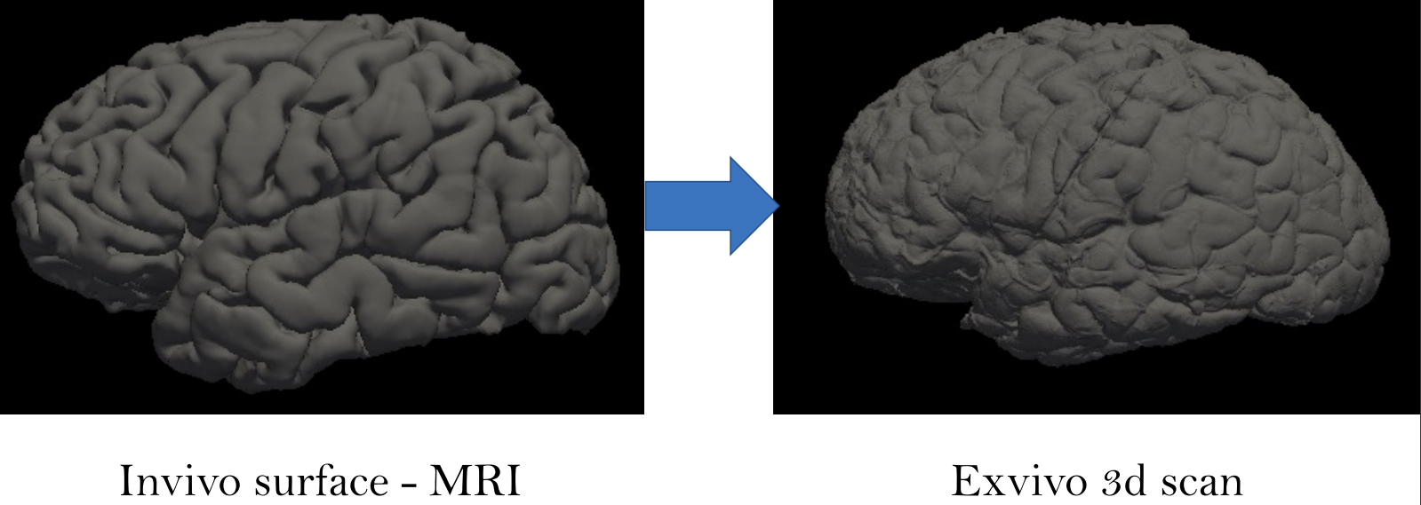
Ex-vivo surface mesh reconstruction from in-vivo FreeSurfer meshes is a process used to construct 3D models of neurological structures. This entails translating in-vivo MRI FreeSurfer meshes into higher-quality ex-vivo meshes. To accomplish this, the brain is first removed from the skull and placed in a solution to prevent deformation. A high-resolution MRI scanner produces a detailed 3D model of the brain’s surface.  The in-vivo FreeSurfer mesh and the ex-vivo model are integrated for analysis and visualization, making this process beneficial for exploring brain structures, thereby helping scientists learn how it functions.

2. Approach

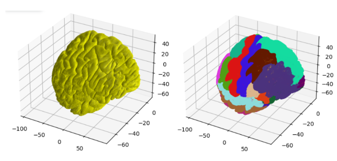
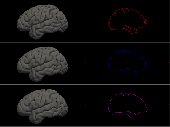
This project aims to construct anatomically accurate ex-vivo surface models of the brain from in-vivo FreeSurfer meshes. The source code for our project can be found in this GitHub repo. A software tool called FreeSurfer can be used to produce cortical surface representations from structural MRI data. However, because of distortion and shrinking, these meshes do not adequately depict the exact shape of the brain once it is removed from the skull. As a result, we propose a method for producing more realistic ex-vivo meshes for anatomical investigations and comparisons. For this task, we used five in-vivo meshes which were provided along with their annotations.  Figure 2 shows a sample in-vivo mesh and its annotation.

We attempted to solve this using two different spaces: 

1. Volumetric space
2. Surface space

 2.1. Volumetric Space

Our volumetric method consists of the following steps:

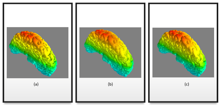
1.  First, we fill in the high-resolution mesh into a 3D volume. This process ensures that the fine details of the cortical surface, such as gyri and sulci, are preserved while avoiding holes or gaps in the mesh. We performed the filling operation at three different resolutions which are 3,4 and 5 using FreeSurfer’s “mris_fill” command.

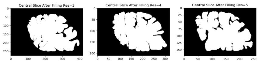
2. The deep sulci of the brain are then closed. Sulci are the grooves or fissures in the brain that separate the gyri or ridges. These sulci can sometimes be overly deep or too wide, affecting the quality of brain imaging or analysis. This step is necessary because in-vivo meshes often include open sulci which are not visible in the ex-vivo condition due to tissue collapse and folding. By closing the sulci, we can obtain a smoother and more compact mesh that resembles the ex-vivo brain surface.

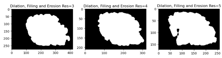
3. Morphological operations are methods that change the shape or structure of a shape depending on a preset kernel or structuring element. There are a number of morphological operations, but we will concentrate on three here: dilation, fill and erode. Dilation extends an object’s borders by adding pixels to its edges. Fill adds pixels to the interior of an object to fill in any holes or gaps. Erode reduces the size of an object’s bounds by eliminating pixels from its edges. We can apply morphological operations to smooth out the brain surface and close the gaps to remedy this problem.

We used the following operations in a specified order to close the deep sulci of the brain: dilation, fill and erode. We first dilate the brain image to make the sulci smaller and less deep. The remaining spaces in the sulci are then filled to make them disappear. Finally, the brain image is eroded to recover its original size and shape. As a result, the brain surface is smoother and more uniform, with no deep sulci. 

4. The extraction of iso-surfaces from the three-dimensional volumetric data is accomplished using the well-known algorithm Marching Cubes, which results in a more uniform and accurate representation of the brain surface. This process transforms the three-dimensional volume into a surface mesh that can be visualized and examined.  

5. Then we used the Gaussian smoothing algorithm in order to smooth the output of the marching cubes algorithm. In order to smooth an image, a Gaussian function is applied to each pixel using a Gaussian blur filter. Often employed in statistics, the normal distribution is mathematically described by a function called a Gaussian function. A Gaussian function in one dimension has the following form:

Figure 4 shows the visualization results of the reconstruction results before and after the application of Gaussian smoothing.

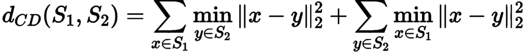
6. Finally, we used the density-aware chamfer distance to assess the quality of the reconstructed mesh. For comparing point sets, two popular metrics known as Chamfer Distance (CD) and Earth Mover’s Distance (EMD) are commonly used. While EMD focuses on global distribution and disregards fine-grained structures, CD does not take into account local density variations, potentially disregarding the underlying similarity between point sets with various density and structure features. We define the chamfer distance between two pointsets using the formula below:

From the reconstruction results, we can visually see that when the resolution increases the result is not so great. After performing the morphological operations we can see that the results for resolution of 5 still have some holes and the sulci is still deep. While for the lowest resolution of 3, we can see that the reconstruction is closer to ex-vivo than in-vivo. In order to validate our assumptions from the visualization, we computed the chamfer distance between the original mesh and the reconstructed mesh after the morphological operations are performed. The results after the calculation are summarized in Table 1. 

Resolutions	N=10	N=100	N=1000	N=10000
3	4.15	7.62	76.26	274.73
4	5.66	10.09	42.92	182.66
5	4.53	8.60	33.19	168.83

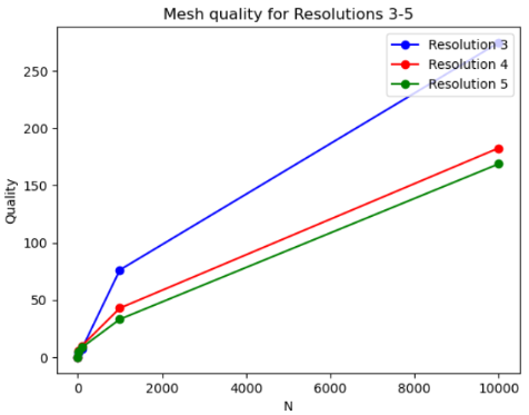
After getting the point clouds from both meshes, we only considered a subset of the vertices to compute the distance since considering the entire point cloud is computationally intensive and very slow. We took the number of vertices to be powers of 10. Then the point clouds were rescaled and normalized to be in the same space. From the results, we can conclude that the higher resolution has the lowest distance, while the lowest resolution has the highest distance. This is true from our observation that the highest resolution should be closer to the original mesh while the lowest resolution is further from it since it’s getting similar to an ex-vivo mesh. Figure 8 shows a plot of the mesh quality for the different resolutions, where the number of vertices is given on the x-axis and the distance is given on the y-axis.

2.2. Surface-based approach

Sellán et al. demonstrate in “Opening and Closing Surfaces (2020)” that many regions don’t move when performing closing operations, and the output is curvature bound, as shown in Figure 9.

Therefore, Sellán et al. propose a bounded curvature-based flow for 3D surfaces that moves not curvature bound points in the normal direction by an amount proportional to their curvature.

As an alternative to the volumetric closing of the deep sulci of the brain, we applied the Sellán et al. method to close our surfaces. Figures 10 and 11 present the progressive closing of the mesh at each iteration until it converges.

2.3. Extracting External Surface

One other approach we tried to explore was focused on getting only the outer surface without all the grooves by post-processing the meshes reconstructed from the in-vivo reconstructed surface (Figure 12. a). So we followed the following steps:

1. Inflate the mesh by pushing each vertex in the direction of its normals. This results in the closing of all the grooves and only the external surface is directly visible. The inflated mesh is shown in Figure 12. b
2. Once we have this inflated surface, we need to retrieve only the externally visible surface. For this, we treat all the brain vertex as origins and shoot rays in the direction of vertex normals. The rays originating from vertices lying on the external surface do not hit any other surface, whereas the ones from the inside surface hit the external surface. Thus we can find and isolate the vertices lying on the surface. We reconstruct the surface using these extracted meshes using Poisson reconstruction. The reconstructed mesh is shown in Figure 12. c

3. Future work

In this study, we presented a technique for reconstructing an ex-vivo mesh from an in-vivo mesh utilizing various methods. But there are still limitations and difficulties that we would like to address in our future studies. One of them is to mimic the effects of cuts and veins, which are common artifacts in histological images, on the surface of the brain. To achieve this, we intend to produce accurate displacement maps that can simulate the deformation of the brain surface as a result of these factors. Additionally, using displacement maps, we will investigate various techniques for producing random continuous curves on the 2D surface that can depict cuts and veins. Another challenge is to improve the robustness of our method to surface deformation caused by different slicing methods or imaging modalities. We also want to train deep learning networks such as GCN/DiffusionNet to segment different brain regions. We will investigate the use of chamfer distance as a loss function to measure the similarity between the predicted and ground truth segmentation masks, and to encourage smoothness and consistency of the segmentation results across different slices.