Students: Tewodros (Teddy) Tassew, João Pedro Vasconcelos Teixeira, Shanthika Naik, and Sanjana Adapala
TAs: Andrew Rodriguez
Mentor: Karthik Gopinath
1. Introduction
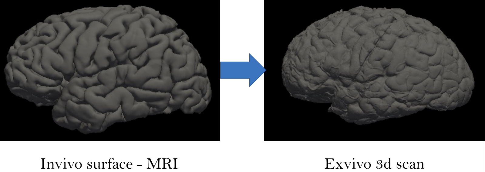
Ex-vivo surface mesh reconstruction from in-vivo FreeSurfer meshes is a process used to construct 3D models of neurological structures. This entails translating in-vivo MRI FreeSurfer meshes into higher-quality ex-vivo meshes. To accomplish this, the brain is first removed from the skull and placed in a solution to prevent deformation. A high-resolution MRI scanner produces a detailed 3D model of the brain’s surface. The in-vivo FreeSurfer mesh and the ex-vivo model are integrated for analysis and visualization, making this process beneficial for exploring brain structures, thereby helping scientists learn how it functions.
Figure 1 Converting in-vivo surface to exvivo 3d scan
2. Approach
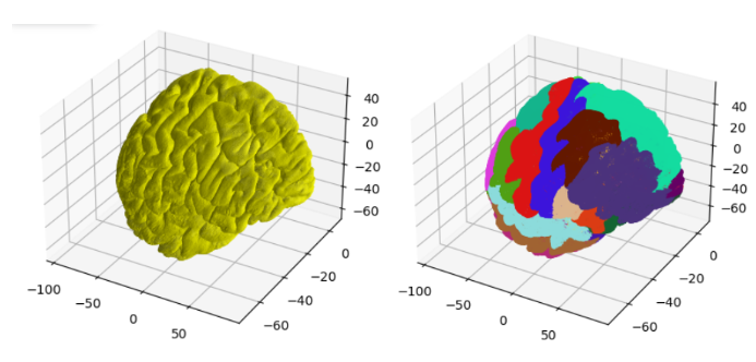
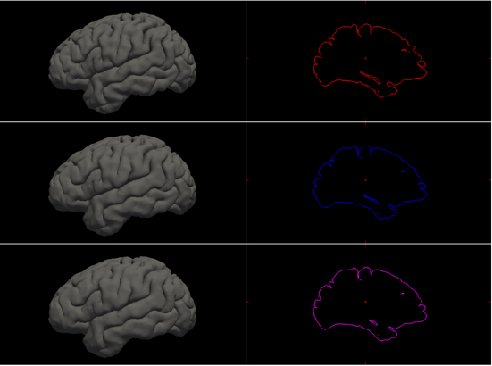
This project aims to construct anatomically accurate ex-vivo surface models of the brain from in-vivo FreeSurfer meshes. The source code for our project can be found in this GitHub repo. A software tool called FreeSurfer can be used to produce cortical surface representations from structural MRI data. However, because of distortion and shrinking, these meshes do not adequately depict the exact shape of the brain once it is removed from the skull. As a result, we propose a method for producing more realistic ex-vivo meshes for anatomical investigations and comparisons. For this task, we used five in-vivo meshes which were provided along with their annotations. Figure 2 shows a sample in-vivo mesh and its annotation.
Figure 2 Sample in-vivo mesh and its annotation
We attempted to solve this using two different spaces:
Volumetric space
Surface space
2.1. Volumetric Space
Our volumetric method consists of the following steps:
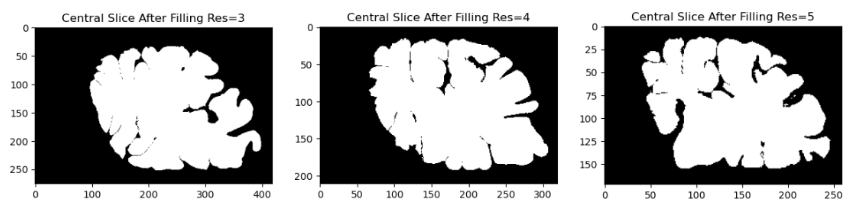
First, we fill in the high-resolution mesh into a 3D volume. This process ensures that the fine details of the cortical surface, such as gyri and sulci, are preserved while avoiding holes or gaps in the mesh. We performed the filling operation at three different resolutions which are 3,4 and 5 using FreeSurfer’s “mris_fill” command.
Figure 3 Central slice for different resolutions after filling
The deep sulci of the brain are then closed. Sulci are the grooves or fissures in the brain that separate the gyri or ridges. These sulci can sometimes be overly deep or too wide, affecting the quality of brain imaging or analysis. This step is necessary because in-vivo meshes often include open sulci which are not visible in the ex-vivo condition due to tissue collapse and folding. By closing the sulci, we can obtain a smoother and more compact mesh that resembles the ex-vivo brain surface.
Figure 4 Central slice for different resolutions after closing
Morphological operations are methods that change the shape or structure of a shape depending on a preset kernel or structuring element. There are a number of morphological operations, but we will concentrate on three here: dilation, fill and erode. Dilation extends an object’s borders by adding pixels to its edges. Fill adds pixels to the interior of an object to fill in any holes or gaps. Erode reduces the size of an object’s bounds by eliminating pixels from its edges. We can apply morphological operations to smooth out the brain surface and close the gaps to remedy this problem.
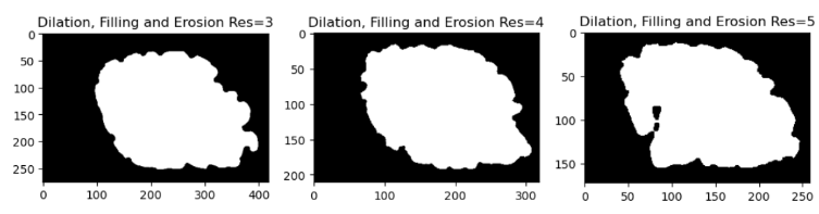
We used the following operations in a specified order to close the deep sulci of the brain: dilation, fill and erode. We first dilate the brain image to make the sulci smaller and less deep. The remaining spaces in the sulci are then filled to make them disappear. Finally, the brain image is eroded to recover its original size and shape. As a result, the brain surface is smoother and more uniform, with no deep sulci.
Figure 5 Central slice for different resolutions after dilation, filling, and erosion
The extraction of iso-surfaces from the three-dimensional volumetric data is accomplished using the well-known algorithm Marching Cubes, which results in a more uniform and accurate representation of the brain surface. This process transforms the three-dimensional volume into a surface mesh that can be visualized and examined.
Then we used the Gaussian smoothing algorithm in order to smooth the output of the marching cubes algorithm. In order to smooth an image, a Gaussian function is applied to each pixel using a Gaussian blur filter. Often employed in statistics, the normal distribution is mathematically described by a function called a Gaussian function. A Gaussian function in one dimension has the following form:
Figure 4 shows the visualization results of the reconstruction results before and after the application of Gaussian smoothing.
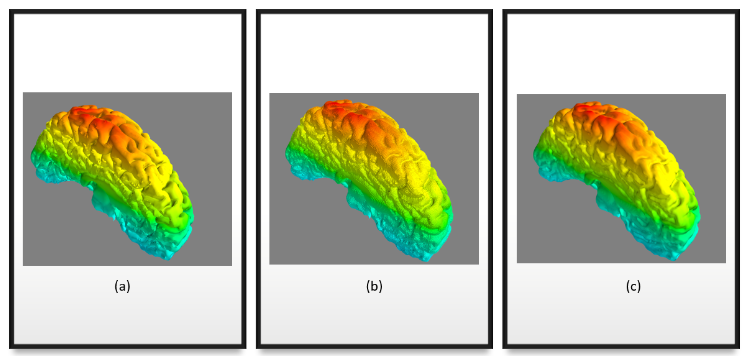
Figure 7 (a) original mesh, (b) reconstructed mesh using marching cubes without smoothing, (c) reconstructed mesh after smoothing.
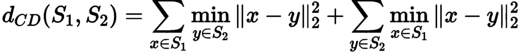
Finally, we used the density-aware chamfer distance to assess the quality of the reconstructed mesh. For comparing point sets, two popular metrics known as Chamfer Distance (CD) and Earth Mover’s Distance (EMD) are commonly used. While EMD focuses on global distribution and disregards fine-grained structures, CD does not take into account local density variations, potentially disregarding the underlying similarity between point sets with various density and structure features. We define the chamfer distance between two pointsets using the formula below:
From the reconstruction results, we can visually see that when the resolution increases the result is not so great. After performing the morphological operations we can see that the results for resolution of 5 still have some holes and the sulci is still deep. While for the lowest resolution of 3, we can see that the reconstruction is closer to ex-vivo than in-vivo. In order to validate our assumptions from the visualization, we computed the chamfer distance between the original mesh and the reconstructed mesh after the morphological operations are performed. The results after the calculation are summarized in Table 1.
Resolutions
N=10
N=100
N=1000
N=10000
3
4.15
7.62
76.26
274.73
4
5.66
10.09
42.92
182.66
5
4.53
8.60
33.19
168.83
Table 1 Chamfer distance for different resolutions
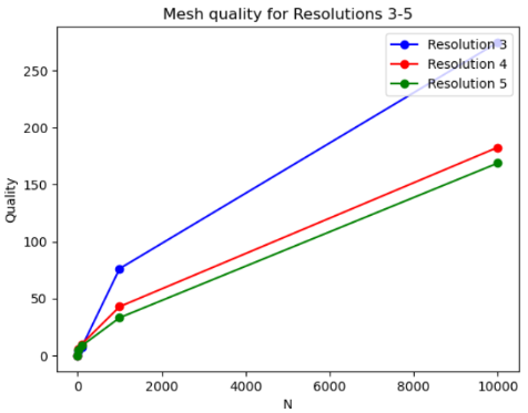
After getting the point clouds from both meshes, we only considered a subset of the vertices to compute the distance since considering the entire point cloud is computationally intensive and very slow. We took the number of vertices to be powers of 10. Then the point clouds were rescaled and normalized to be in the same space. From the results, we can conclude that the higher resolution has the lowest distance, while the lowest resolution has the highest distance. This is true from our observation that the highest resolution should be closer to the original mesh while the lowest resolution is further from it since it’s getting similar to an ex-vivo mesh. Figure 8 shows a plot of the mesh quality for the different resolutions, where the number of vertices is given on the x-axis and the distance is given on the y-axis.
Figure 8 Mesh quality for different resolutions
2.2. Surface-based approach
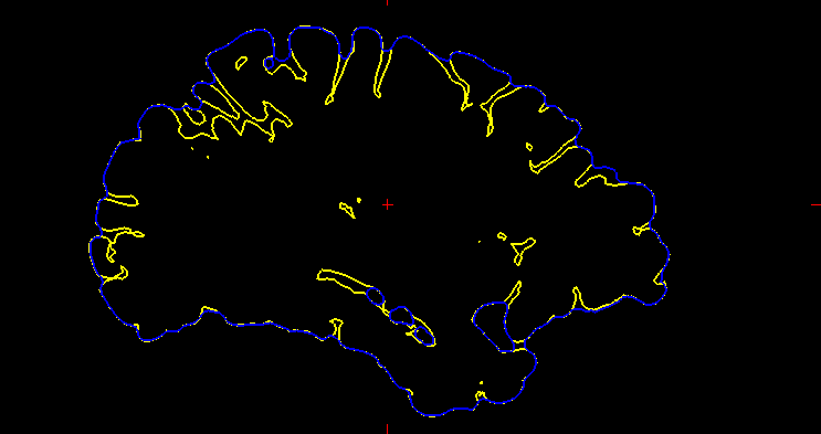
Sellán et al. demonstrate in “Opening and Closing Surfaces (2020)” that many regions don’t move when performing closing operations, and the output is curvature bound, as shown in Figure 9.
Figure 9 (yellow) Original outline, (blue) Closed outline
Therefore, Sellán et al. propose a bounded curvature-based flow for 3D surfaces that moves not curvature bound points in the normal direction by an amount proportional to their curvature.
As an alternative to the volumetric closing of the deep sulci of the brain, we applied the Sellán et al. method to close our surfaces. Figures 10 and 11 present the progressive closing of the mesh at each iteration until it converges.
Figure 10 Surface at each iteration of the closing flow
Figure 11 Outlining the difference at iterations 2, 4 and 6
2.3. Extracting External Surface
One other approach we tried to explore was focused on getting only the outer surface without all the grooves by post-processing the meshes reconstructed from the in-vivo reconstructed surface (Figure 12. a). So we followed the following steps:
Inflate the mesh by pushing each vertex in the direction of its normals. This results in the closing of all the grooves and only the external surface is directly visible. The inflated mesh is shown in Figure 12. b
Once we have this inflated surface, we need to retrieve only the externally visible surface. For this, we treat all the brain vertex as origins and shoot rays in the direction of vertex normals. The rays originating from vertices lying on the external surface do not hit any other surface, whereas the ones from the inside surface hit the external surface. Thus we can find and isolate the vertices lying on the surface. We reconstruct the surface using these extracted meshes using Poisson reconstruction. The reconstructed mesh is shown in Figure 12. c
Figure 12 Post-processing the meshes reconstructed from the in-vivo reconstructed surface
3. Future work
In this study, we presented a technique for reconstructing an ex-vivo mesh from an in-vivo mesh utilizing various methods. But there are still limitations and difficulties that we would like to address in our future studies. One of them is to mimic the effects of cuts and veins, which are common artifacts in histological images, on the surface of the brain. To achieve this, we intend to produce accurate displacement maps that can simulate the deformation of the brain surface as a result of these factors. Additionally, using displacement maps, we will investigate various techniques for producing random continuous curves on the 2D surface that can depict cuts and veins. Another challenge is to improve the robustness of our method to surface deformation caused by different slicing methods or imaging modalities. We also want to train deep learning networks such as GCN/DiffusionNet to segment different brain regions. We will investigate the use of chamfer distance as a loss function to measure the similarity between the predicted and ground truth segmentation masks, and to encourage smoothness and consistency of the segmentation results across different slices.
Students: Tewodros (Teddy) Tassew, Anthony Ramos, Ricardo Gloria, Badea Tayea
TAs: Heng Zhao, Roger Fu
Mentors: Yingying Wu, Etienne Vouga
Introduction
Shape analysis has been an important topic in the field of geometry processing, with diverse interdisciplinary applications. In 2005, Reuter, et al., proposed spectral methods for the shape characterization of 3D and 2D geometrical objects. The paper demonstrates that the Laplacian operator spectrum is able to capture the geometrical features of surfaces and solids. Besides, in 2006, Reuter, et al., proposed an efficient numerical method to extract what they called the “Shape DNA” of surfaces through eigenvalues, which can also capture other geometric invariants. Later, it was demonstrated that eigenvalues can also encode global properties like topological features of the objects. As a result of the encoding power of eigenvalues, spectral methods have been applied successfully to several fields in geometry processing such as remeshing, parametrization and shape recognition.
In this project, we present a discrete surface characterization method based on the extraction of the top smallest k eigenvalues of the Laplace-Beltrami operator. The project consists of three main parts: data preparation, geometric feature extraction, and shape classification. For the data preparation, we cleaned and remeshed well-known 3D shape model datasets; in particular, we processed meshes from ModelNet10, ModelNet40, and Thingi10k. The extraction of geometric features is based on the “Shape DNA” concept for triangular meshes which was introduced by Reuter, et al. To achieve this, we computed the Laplace-Beltrami operator for triangular meshes using the robust-laplacian Python library.
Finally, for the classification task, we implemented some machine learning algorithms to classify the smallest k eigenvalues. We first experimented with simple machine learning algorithms like Naive Bayes, KNN, Random Forest, Decision Trees, Gradient Boosting, and more from the sklearn library. Then we experimented with the sequential model Bidirectional LSTM using the Pytorch library to try and improve the results. Each part required different skills and techniques, some of which we learned from scratch and some of which we improved throughout the two previous weeks. We worked on the project for two weeks and received preliminary results. The GitHub repo for this project can be found in this GitHub repo.
Data preparation
The datasets used for the shape classification are:
1. ModelNet10: The ModelNet10 dataset, a subset of the larger ModelNet40 dataset, contains 4,899 shapes from 10 categories. It is pre-aligned and normalized to fit in a unit cube, with 3,991 shapes used for training and 908 shapes for testing.
2. ModelNet40: This widely used shape classification dataset includes 12,311 shapes from 40 categories, which are pre-aligned and normalized. It has a standard split of 9,843 shapes for training and 2,468 for testing, making it a widely used benchmark.
3. Thingi10k: Thingi10k is a large-scale dataset of 10,000 models from thingiverse.com, showcasing the variety, complexity, and quality of real-world models. It contains 72 categories that capture the variety and quality of 3D printing models.
For this project, we decided to use a subset of the ModelNet10 dataset to perform some preprocessing steps on the meshes and apply a surface classification algorithm due to the number of classes it has for analysis. Meanwhile, the ModelNet10 dataset is unbalanced, so we selected 50 shapes for training and 25 for testing per class.
Moreover, ModelNet datasets do not fully represent the surface representations of objects; self-intersections and internal structures are present, which could affect the feature extraction and further classification. Therefore, for future studies, a more careful treatment of mesh preprocessing is of primary importance.
Preprocessing Pipeline
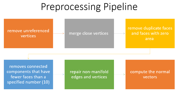
After the dataset preparation, the preprocessing pipeline consists of some steps to clean up the meshes. These steps are essential to ensure the quality and consistency of the input data, and to avoid errors or artifacts. We used the PyMeshLab library, which is a Python interface to MeshLab, for mesh processing. The pipeline consists of the following steps:
1.Remove unreferenced vertices: This method gets rid of any vertices that don’t belong to a face.
2. Merge nearby vertices: This function combines vertices that are placed within a certain range (i.e., ε = 0.001).
3.Remove duplicate faces and faces with zero areas: It eliminates faces with the same features or no area.
4. Removes connected components that have fewer faces than a specified number (i.e. 10): The effectiveness and accuracy of the model can be enhanced by removing isolated mesh regions that are too small to be useful.
5.Repair non-manifold edges and vertices: It corrects edges and vertices that are shared by more than two faces, which is a violation of the manifold property. The mesh representation can become problematic with non-manifold geometry.
6.Compute the normal vectors: The orientation of the adjacent faces is used to calculate the normal vectors for each mesh vertex.
These steps allow us to obtain clean and consistent meshes that are ready for the remeshing process.
Figure 1 Preprocessing Pipeline
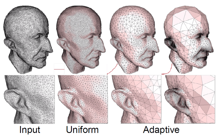
Adaptive Isotropic Remeshing
The quality of the meshes is one of the key problems with the collected 3D models. When discussing triangle quality, it’s important to note that narrow triangles might result in numerical inaccuracies when the Laplace-Beltrami operator is being computed. In that regard, we remeshed each model utilizing adaptive isotropic remeshing implemented in PyMeshLab. Triangles with a favorable aspect ratio can be created using the procedure known as isotropic remeshing. In order to create a smooth mesh with the specified edge length, the technique iteratively carries out simple operations like edge splits, edge collapses, and edge flips.
Adaptive isotropic remeshing transforms a given mesh into one with non-uniform edge lengths and angles, maintaining the original mesh’s curvature sensitivity. It computes the maximum curvature for the reference mesh, determines the desired edge length, and adjusts split and collapse criteria accordingly. This technique also preserves geometric details and reduces the number of obtuse triangles in the output mesh.
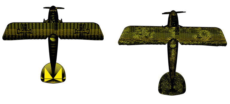
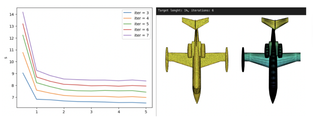
We applied the PyMeshLab function ms.meshing_isotropic_explicit_remeshing() to remesh the ModelNet10 dataset for this project. We experimented with different parameters of the isotropic remeshing algorithm from PyMeshLab to optimize the performance. The optimal parameters for time, type of remesh, and triangle quality were iterations=6, adaptive=True, and targetlen=pymeshlab.Percentage(1) respectively. The adaptive=True parameter enabled us to switch from uniform to adaptive isotropic remeshing. Figure 3 illustrates the output of applying adaptive remeshing to the airplane_0045.off mesh from the ModelNet40 training set. We also tried the pygalmesh.remesh_surface() function, but it was very slow and produced unsatisfactory results.
Figure 3 Plot for time vs target length (left) and the yellow airplane is the re-meshing result for parameter values of Iterations = 6 and targetlen = 1% while the blue airplane is the original mesh (right).
The Laplace-Beltrami Spectrum Operator
In this section, we introduce some of the basic theoretical foundations used for our characterization. Specifically, we define the Laplacian-Beltrami operator along with some of its key properties, explain the significance of the operator and its eigenvalues, and display how it has been implemented in our project.
Definition and Properties of the Laplace-Beltrami Operator
The Laplacian-Beltrami operator, often denoted as Δ, is a differential operator which acts on smooth functions on a Riemannian manifold (which, in our case, is the 3D surface of a targeted shape). The Laplacian-Beltrami operator is an extension of the Laplacian operator in Euclidean space, adjusted for curved surfaces on the manifold. Mathematically, the Laplacian-Beltrami operator acting on a function on a manifold is defined using the following formula:
where ∂idenotes the i-th partial derivative, g is the determinant of the metric tensor gij of the manifold and gijis the inverse of the metric tensor.
The Laplacian-Beltrami operator serves as a measure of how the value of f at a point deviates from its average value within infinitesimally small neighborhoods around that point. Therefore, the operator can be adopted to describe the local geometry of the targeted surface.
The Eigenvalue Problem and Its Significance
Laplacian-Beltrami operator is a second-order function applied to a surface, which could be represented as a matrix whose eigenvalues/eigenvectors provide information about the geometry and topology of a surface.
The significance of the eigenvalue problem as a result of applying the Laplace-Beltrami Operator includes:
Functional Representation. The eigenfunctions corresponding to a particular geometric surface form an orthonormal basis of all functions on the surface, providing an efficient way to represent any function on the surface.
Surface Characterization. A representative feature vector containing the eigenvalues creates a “Shape-DNA” of the surface, which captures the most significant variations in the geometry of the surface.
Dimensionality Reduction. Using eigenvalues can effectively reduce the dimensionality of the data used, aiding in more efficient processing and analysis.
Feature Discrimination. The geometric variations and differences between surfaces can be identified using eigenvalues. If two surfaces have different eigenvalues, they are likely to have different geometric properties. Surface eigenvalue analysis can be used to identify features that are unique to each surface. This can be beneficial in computer graphics and computer vision applications where it is necessary to distinguish between different surfaces.
Discrete Representation of Laplacian-Beltrami Operator
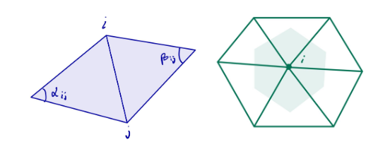
In the discrete setting, the Laplacian-Beltrami operator is defined on the given meshes. The Discrete Laplacian-Beltrami operator L can be defined and computed using different approaches. An often-used representation is using the cotangent matrix defined as follows:
Then L = M-1C where M is the diagonal mass matrix whose i-th entry is the shaded area as shown in Figure 4 for each vertex i. The Laplacian matrix is a symmetric positive-semidefinite matrix. Usually, L is sparse and stored as a sparse matrix in order not to waste memory.
Figure 4 (Left) Definition of edge i-j and angles for a triangle mesh. (Right) Representation of Voronoi area for vertex vi.
A Voronoi diagram is a mathematical method for dividing a plane into areas near a collection of objects, each with its own Voronoi cell. It contains all of the points that are closer to it than any other object. Since its origin, engineers have utilized the Delaunay triangulation to maximize the minimum angle among possible triangulations of a fixed set of points. In a Voronoi diagram, this triangulation corresponds to the nerve cells.
Experimental Results
In our experiments, we rescaled the vertices before computing the cotangent Laplacian. Rescaling mesh vertices changes the size of an object without changing its geometry. This Python function rescales a 3D point cloud by translating it to fit within a unit cube centered at the origin. It then scales the point cloud to have a maximum norm of 1, ensuring its center is at the origin. The function then finds the maximum and minimum values of each dimension in the input point cloud, computes the size of the point cloud in each dimension, and computes a scaling factor for each dimension. The input point cloud is translated to the center at the origin and scaled by the maximum of these factors, resulting in a point cloud with a maximum norm of 1.
Throughout this project, we used the robust-laplacian Python package to compute the Laplacian-Beltrami operator. This library deals with point clouds instead of triangle meshes. Moreover, the package can handle non-manifold triangle meshes by implementing the algorithm described in A Laplacian for Nonmanifold Triangle Meshes by Nicholas Sharp and Keenan Crane.
For the computation of the eigenvalues, we used the SciPy Python library. Let’s recall the eigenvalue problem Lv = λv, where λ is a scalar, and v is a vector. For a linear operator L, we called λ eigenvalue and v eigenvector respectively. In our project, the smallest keigenvalues and eigenfunctions corresponding to 3D surfaces formed feature vectors for each shape, which were then used as input of machine learning algorithms for tasks such as shape classification.
Surface Classification
The goal of this project was to apply spectral methods to surface classification using two distinct datasets: a synthetic one and ModelNet10. We used the Trimesh library to create some basic shapes for our synthetic dataset and performed remeshing on each shape. This was a useful step to verify our approach before working with more complicated data. The synthetic data had 6 classes with 50 instances each. The shapes were Annulus, Box, Capsule, Cone, Cylinder, and Sphere. We computed the first 30 eigenvalues on 50 instances of each class, following the same procedure as the ModelNet dataset so that we could compare the results of both datasets. We split the data into 225 training samples and 75 testing samples.
For the ModelNet10 dataset, we selected 50 meshes for the training set and 25 meshes for the testing set per class. In total, we took 500 meshes for the training set and 250 meshes for the testing set. After experimenting with different machine learning algorithms, the validation results for both datasets are summarized below in Table 1. The metric used for the evaluation procedure is accuracy.
Models
Accuracy for Synthetic Dataset
Accuracy for ModelNet 10
KNN
0.49
0.31
Random forest
0.69
0.33
Linear SVM
0.36
0.11
RBF SVM
0.60
0.10
Gaussian Process
0.59
0.19
Decision Tree
0.56
0.32
Neural Net
0.68
0.10
AdaBoost
0.43
0.21
Naive Bayes
0.23
0.19
QDA
0.72
0.21
Gradient Boosting
0.71
0.31
Table 1 Accuracy for synthetic and ModelNet10 datasets using different machine learning algorithms.
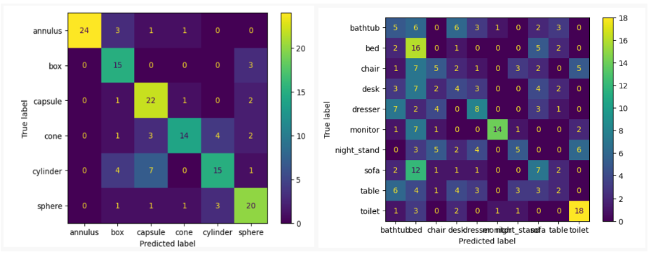
From Table 1 we can observe that the decision tree, random forest, and gradient boosting algorithms performed well on both datasets. These algorithms are suitable for datasets that have graphical features. We used the first 30 eigenvalues on 50 samples of each class for both the ModelNet and synthetic datasets, ensuring a fair comparison between the two datasets. Figure 5 shows the classification accuracy for each class using the confusion matrix.
Figure 5 Confusion matrix using Random Forest on the synthetic dataset (left) and ModelNet10 dataset (right).
We conducted two additional experiments using deep neural networks implemented in Pytorch, besides the machine learning methods we discussed before. The first experiment involved a simple MLP model consisting of 5 fully connected layers, each with the Batch Norm and ReLU activation functions. The model achieved an accuracy of 57% on the synthetic dataset and 15% on the ModelNet10 dataset for the testing set. The second experiment used a sequential model called Bidirectional LSTM with two layers. The model achieved an accuracy of 34% for the synthetic dataset and 33% for the ModelNet10 dataset based on the testing set. These are reasonable results since the ModelNet dataset contains noise, artifacts, and flaws, potentially affecting model accuracy and robustness. Examples include holes, missing components, uneven surfaces, and most importantly, the interior structures. All of these issues could potentially impact the overall performance of the models, especially for our classification purposes. We present the results in Table 2. The results indicate that the MLP model performed well on the synthetic dataset while the Bi-LSTM model performed better on the ModelNet10 dataset.
Models
Accuracy for Synthetic Dataset
Accuracy for ModelNet 10
MLP
0.57
0.15
Bi-LSTM
0.34
0.33
Table 2 Accuracy for synthetic and ModelNet10 datasets using deep learning algorithms.
Future works
We faced some challenges with the ModelNet10 dataset. The dataset had several flaws that resulted in lower accuracy when compared to the synthetic dataset. Firstly, we noticed some meshes with disconnected components, which caused issues with the computation of eigenvalues, since we would get one zero eigenvalue for each disconnected component, lowering the quality of the features computed for our meshes. Secondly, these meshes had internal structures, i.e., vertices inside the surface, which also affected the surface recognition power of the computed eigenvalues, as well as other problems related to self-intersections and non-manifold edges.
The distribution of eigenvalues in a connected manifold is affected by scaling. The first-keigenvalues are related to the direction encapsulating the majority of the manifold’s variation. Scaling by α results in a more consistent shape with less variation along the first-k directions. On the other hand, scaling by 1/α causes the first-k eigenvalues to grow by α2, occupying a higher fraction of the overall sum of eigenvalues. This implies a more varied shape with more variance along the first-k directions.
To address the internal structures problem, we experimented with several state-of-the-art surface reconstruction algorithms for extracting the exterior shape and removing internal structures using the Ball Pivoting, Poisson Distribution methods from the Python PyMeshLab library, and Alpha Shapes. One of the limitations of ball pivoting is that the quality and completeness of the output mesh depend on the choice of the ball radius. The algorithm may miss some parts of the surface or create holes if the radius is too small. Conversely, if the radius is too large, the method could generate unwanted triangles or smooth sharp edges. Ball pivoting also struggles with noise or outliers and can result in self-intersections or non-manifold meshes.
By using only vertices to reconstruct the surface, we significantly reduced the computational time but the drawback was that the extracted surface was not stable enough to recover the entire surface. It also failed to remove the internal structures completely. In future work, we intend to address this issue and create an effective algorithm that can extract the surface from this “noisy” data. For this issue, implicit surface approaches show great promise.
References
Reuter, M., Wolter, F.-E., & Niklas Peinecke. (2005). Laplace-spectra as fingerprints for shape matching. Solid and Physical Modeling. https://doi.org/10.1145/1060244.1060256
Reuter, M., Wolter, F.-E., & Niklas Peinecke. (2006). Laplace–Beltrami spectra as “Shape-DNA” of surfaces and solids. Computer Aided Design, 38(4), 342–366. https://doi.org/10.1016/j.cad.2005.10.011
Reuter, M., Wolter, F.-E., Shenton, M. E., & Niethammer, M. (2009). Laplace–Beltrami eigenvalues and topological features of eigenfunctions for statistical shape analysis. 41(10), 739–755. https://doi.org/10.1016/j.cad.2009.02.007
Nealen, A., Igarashi, T., Sorkine, O., & Alexa, M. (2006). Laplacian mesh optimization. Conference on Computer Graphics and Interactive Techniques in Australasia and Southeast Asia. https://doi.org/10.1145/1174429.1174494
The opening day of the MIT Summer Geometry Initiative 2023 was filled with engagement as the students dived into the world of geometry.
The program kicked off with Dr. Solomon welcoming the 2023 SGI Fellows and provided basic information on how the week will go.
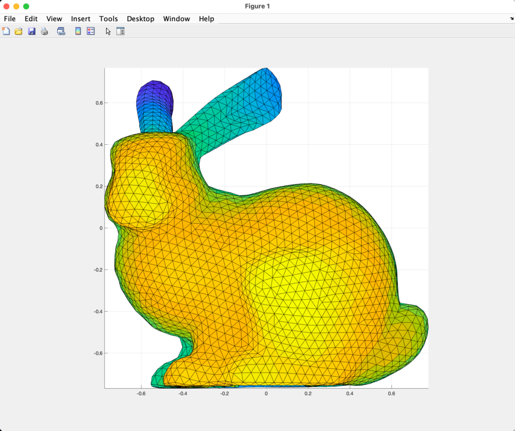
It was followed by Dr. Oded Stein’s course introducing the basic techniques in geometry processing using the gptoolbox library. His talk started with a review of the basic concepts of geometry from the perspectives of different people who might use it. Dr. Stein also introduced the students to some advanced topics, such as how to store surfaces on a computer and how to define the boundary of a surface. The students were given various MATLAB exercises to experiment with the ideas he talked about.
In the afternoon, we had a guest lecture from Dr. Vladmir (Vova) Kim at Adobe, who spoke on the applications of geometry processing. He explained how geometry processing can be used to manipulate shapes in different ways, such as deformation, using neural progressive meshes and parameterization. The methods he introduced can be applied to computer graphics and computer vision. The lecture provided us with a glimpse into state-of-the-art in this cutting-edge field.
Overall, the first day of the MIT Summer Geometry Initiative 2023 was a resounding success. The students left with a solid foundation in geometry processing, ready to tackle more advanced topics in the days ahead.