Fellows: Gizem Altintas, Ikaro Costa, Emi Neuwalder, Kyle Onghai, and Hossam Saeed
Volunteers: Shaimaa Monem and Andrew Rodriguez
Mentor: Frank Yang
Introduction
In geometry processing, mesh simplification refers to a class of algorithms that convert a given polygonal mesh to a new mesh with fewer faces. Typically, the mesh is simplified in a way that optimizes the preservation of specific, user-defined properties like distortion (Hausdorff distance, normals) or appearance (colors, features).

One application of mesh simplification is adapting high-detail art assets for real-time rendering. Unfortunately, when applying common mesh decimation techniques based on iterated local edge collapse, the resulting mesh can be difficult to edit; local edge collapse and edge flip techniques often do not preserve edge loops or have irregular shading and deformation artifacts.
On the other hand, quad mesh simplification methods like polychord collapse can retain more of the edge loop structure of the original mesh at the cost of more complexity. For example, polychord collapse uses non-local operations on sequences of quads (polychords), and quad remeshing even requires global optimization and reconstruction.
Is there a simpler way that allows us to preserve these edge loops throughout simplification while limiting ourselves to local operations, i.e. edge collapses, flips, and regularization? The original quad mesh might provide a starting point as it seems to define a frame field at most points on the mesh that we can use to perhaps guide our local operations.
The potential benefit of this is we can obtain nicely tessellated quad meshes from either quad meshes or even a not-so-nice triangle mesh without having to resort to more complex techniques such as quad polychord collapse or quad remeshing.
Triangle mesh simplification
The first question one might ask is why do the standard triangular decimation techniques often fail to retain edge loops. We would retort, “Why should they?” There is no mechanism that would coerce standard triangular decimation techniques to preserve edge loops. To convince you of this, we will delve into how the quadric error metric (QEM) mesh simplification method of Garland and Heckbert, one of the most well-known triangular mesh simplification algorithms and the one upon which we have built our own, works.
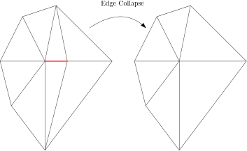
The fundamental operation in Garland and Heckbert’s QEM algorithm is edge collapse, hence its classification as an iterated edge collapse method. As shown in Figure 1, collapsing an edge involves fusing two pendant vertices of an edge. In some cases, we may find it interesting to merge vertices that are not joined by an edge in spite of the possibility of non-manifold (“non-3D-printable”) meshes arising.
Mesh simplification algorithms rooted in iterated edge collapse all boil down to how to decide which edge should be removed at each step. This is facilitated through a cost function, which is an indicator of how much the geometry of the mesh changes when an edge is collapsed. We summarize the algorithm with the following deceptively simple set of instructions.
- For each edge, store the cost of a collapse in a priority queue.
- Collapse the cheapest edge. That is, we remove the cheapest edge and all adjacent triangles and merge the pendant edges of this edge. The position of the merged vertex may be distinct from those of its ancestors.
- Recalculate the cost for all edges altered by the collapse and reorder them within the priority queue.
- Repeat from 2 until the stop condition is met.
Quadric error metrics
We now turn to Garland and Heckbert used QEM’s to define a cost function. Suppose we are given a plane in 3D space specified by a normal \(\mathbf{n}\in \mathbf{R}^3\) and the distance of the plane from the origin \(d\in \mathbf{R}\). We can determine the squared distance to a point \(p\) as follows:
\begin{align*}
Q(\mathbf{p}) &= (\mathbf{p}\cdot \mathbf{n} – d)^2 \\
&= ( \mathbf{p}^{\mathsf{T}} \mathbf{n} – d ) ( \mathbf{n}^{\mathsf{T}} \mathbf{p} – d ) \\
&= \mathbf{p}^{\mathsf{T}} A \mathbf{p} + \mathbf{b}^{\mathsf{T}} \mathbf{p} + d^2
\end{align*}
where \(A = \mathbf{n} \mathbf{n}^{\mathsf{T}}\) and \(\mathbf{b} = -2d \mathbf{n}\). If we compute $d$ from a point, call it \(\mathbf{p}_0\), in a triangle used to define the plane, then \(d = \mathbf{n}\cdot \mathbf{p}_0\).
So we now have a quadratic function $Q$ called the quadratic error metric represented by the triple $\langle A, \mathbf{b}, d\rangle$. It is also possible to equivalently represent a quadric as a 4×4 matrix via homogeneous coordinates. Measuring the sum of squared distances is straightforward even when we introduce more planes.
\begin{align*}
Q_1(\mathbf{p}) + Q_2(\mathbf{p}) &= \sum_{i=1}^2 \mathbf{p}^{\mathsf{T}} A_i \mathbf{p} + \mathbf{b}_i^{\mathsf{T}} \mathbf{p} + d_i^2 \\
&= \mathbf{p}^{\mathsf{T}} (A_1 + A_2+ \mathbf{p} + \left( \mathbf{b}_1^{\mathsf{T}} + \mathbf{b}_2^{\mathsf{T}} \right) \mathbf{p} + \left( d_1^2 + d_2^2 \right).
\end{align*}
In other words,
$$
Q = Q_1 + Q_2 = \langle A_1 + A_2, b_1 + b_2, d_1 + d_2 \rangle.
$$
In mesh simplification, we compute a QEM for each vertex by summing that for the planes of all incident triangles. We then calculate Q, a QEM for each edge, by summing the QEMs of the endpoints. The cost of collapsing an edge is then \(Q(\mathbf{p})\) where \(\mathbf{p}\) is the position of a collapsed vertex. There are a few ways to place a collapsed vertex. One simple one is to take the position of one of the end-points \(\mathbf{v}_1\) or \(\mathbf{v}_2\) depending on whether \(Q(\mathbf{v}_1) < Q(\mathbf{v}_2)\). We instead optimally place \(\mathbf{p}\). As \(Q\) is a quadratic, its minimum is where \(\nabla Q = 0\), so solving the gradient
$$
\nabla Q(\mathbf{p}) = 2A \mathbf{p} + \mathbf{b}
$$
for \(\mathbf{p}\) gives us
$$
\nabla Q \left( \mathbf{p}^* \right) = 2A\mathbf{p}^* + \mathbf{b} = 0 \text{ implies } \mathbf{p}^* = -\frac{1}{2} A^{-1} \mathbf{b}.
$$
Life is not so simple however. \(A\) may not be full rank, e.g. when all the faces contributing to \(Q\) lie on the same plane \(Q = 0\) everywhere on the plane. In such cases we use the singular value decomposition \(A = U \Sigma V^{\mathsf{T}}\) to obtain the pseudoinverse \(A^{\dagger} = V \Sigma^{\dagger} U^{\mathsf{T}}\) with small singular values set to zero to ensure stability.
In any case, once the new vertex position \(\mathbf{p}’\) and its cost \(Q(\mathbf{p}’)\) are found, we store this data in a priority queue. Then we collapse the cheapest edge, place the new merged vertex appropriately, assign a QEM to the merged vertex by summing those of its ancestors, and update and reinsert the QEM’s of all the neighbors of the merged vertex.
Throughout our discussion, notice that there is no condition on the edge loops. Basing the cost function solely on QEM’s does not account for the edge loops, so we must modify it in order to do so. Our idea is to place a frame field on our mesh that indicates preferred directions we would like to collapse an edge along in order to preserve the edge loop structure.
Our contributions
Frame fields
A frame field as introduced by Panozzo et al. is a vector field that assigns to each point on a surface a pair of possibly non-orthogonal, non-unit-length vectors in the tangent plane as well as their opposite vectors. This is a generalization of a cross field, a kind of vector field that has been introduced before frame fields, in the sense that the tangent vectors must be orthogonal and unit-length.
The purpose of both frame and cross fields are to guide automatic quadrangulation methods for triangle meshes, i.e. methods that convert triangle meshes to quadrilateral meshes. Although many field-guided quadrangulation algorithms have been based on fields derived from the surface geometry, in particular its curvature, recent work of Dielen et al. have considered the question of generating fields that produce quadrilateral meshes that mimic what a professional artist would create, e.g. the output meshes have correctly placed edge loops and do not have irregular shading or deformation artifacts. In future work, we hope we can implement this new research to create frame fields that guide our simplification method. Currently, we use a cross field dictated by the principal curvature directions. To describe how our method combines QEMs with alignment to a frame field, we introduce our novel alignment metric.
Alignment Metric
Suppose we are have a point \(x\) on mesh, \(v\) and \(w\) are vectors in the tangent plane that represent the frame field at \(x\), and $p$ is another vector that represents the (orthogonal) projection of an edge emanating from \(x\) that belongs to the mesh. If \(u\) is the bisector of \(\angle vxw\), then, from high school geometry, the orthogonal line \(u^{\perp}\) is also the bisector of \(\angle -vxw\). Intuitively, if \(p\in \operatorname{span} \{u\} \cup \operatorname{span} \{ u^{\perp} \}\), then \(p\) is as “worst” aligned as is possible. So, if \(\theta = \angle pxu\), we would like to find a function \(f\colon [0,\pi]\to [0,1]\) such that \(f(\theta) = 1\) if \(p\in \operatorname{span}{u}\) and \(f(\theta)=0\) if \(p\in \operatorname{span} \{v\}\cup \operatorname{span} \{w\}\), and our cost function for the incremental simplification algorithm should minimize \(f\) among other factors.
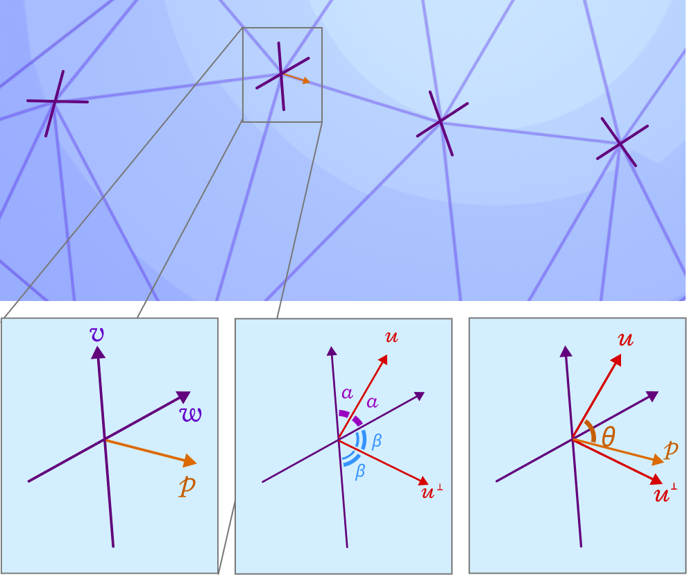
So, if \(\alpha = \angle vxu\) and \(\beta = \angle u^{\perp}xw\), then an example alignment function that is differentiable is
$$
f(\theta) = \begin{cases}
\cos^2 \left( \frac{\pi}{2\alpha} \theta \right) &\text{ if } 0\leq \theta\leq \alpha \\
\cos^2 \left( \frac{\pi}{2\beta} \left( \theta – \frac{\pi}{2} \right) \right) &\text{ if } \alpha\leq \theta\leq \alpha+2\beta \\
\cos^2 \left( \frac{\pi}{2\beta} \left( \theta – \frac{\pi}{2} \right) \right) &\text{ if } \alpha+2\beta\leq \theta\leq \pi
.\end{cases}
$$
With the alignment function in hand, we would like to add it as an additional weight within the cost function of an incremental triangle-based mesh simplification algorithm. We do this simply by multiplying the QEMs by the alignment metric evaluated at the edge that we’re attempting to collapse. For more details, our open source implementation in libigl can be found here. In order to avoid artifacts in the simplified meshes, we have found it helpful to add a small factor, i.e. +1, to the alignment metric.
Results and Future Work
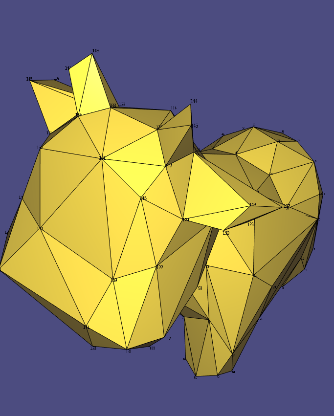
Our results demonstrate that our field-guided, QEM-based mesh simplification method maintains features with high curvature better than Garland and Heckbert’s QEM method. For instance, in the side-by-side comparison below, the ears and horns of Spot in our method (right) have more detail than those in the standard technique of Garland and Heckbert (left).

However, our method in its current iteration still does not preserve edge loop structure and avoid shading irregularities and deformation artifacts to a degree that enable artists to easily edit a simplified mesh. Still, our work is promising in light of the fact that our method simplifies along a frame field not optimized for this purpose, instead prioritizing the surface geometry. We believe that our goal can be achieved by using a frame field generated by the neural method of Dielen et al.
Edge Flips based on Alignment
One idea we still want to build and test out is using edge-flips for getting better edge-loops. Specifically, after each edge-collapse, we look at the one-ring neighborhood of the vertex resulting from the collapsed edge. There, we check all current incident edges and ones that would be incident if an edge-flip is to be applied to one of the vertex’s opposite edges. Finally, the four edges of this set that are best aligned with frame field four directions are selected. Among which, if any of them would result from an edge flip, then we apply it. The animation below shows what the alignment metric of the set of edges with one arbitrary direction looks like.
We initially used a simple dot product for testing alignment, but it seems promising to use the alignment metric discussed earlier and compare the results.
References
Bærentzen, Jakob Andreas, et al. Guide to Computational Geometry Processing. Springer, 2012. DOI.org (Crossref), https://doi.org/10.1007/978-1-4471-4075-7.
Dielen, Alexander, et al. “Learning Direction Fields for Quad Mesh Generation.” Computer Graphics Forum, vol. 40, no. 5, Aug. 2021, pp. 181–91. DOI.org (Crossref), https://doi.org/10.1111/cgf.14366.
Garland, Michael and Paul S. Heckbert. “Surface simplification using quadric error metrics.” Proceedings of the 24th annual conference on Computer graphics and interactive techniques (1997): n. Pag.
Panozzo, Daniele, et al. “Frame Fields: Anisotropic and Non-Orthogonal Cross Fields.” ACM Transactions on Graphics, vol. 33, no. 4, July 2014, p. 134:1-134:11. ACM Digital Library, https://doi.org/10.1145/2601097.2601179.