Fellows: Gizem Altintas, Ikaro Costa, Emi Neuwalder, Kyle Onghai, and Hossam Saeed Volunteers: Shaimaa Monem and Andrew Rodriguez Mentor: Frank Yang
Introduction
In geometry processing, mesh simplification refers to a class of algorithms that convert a given polygonal mesh to a new mesh with fewer faces. Typically, the mesh is simplified in a way that optimizes the preservation of specific, user-defined properties like distortion (Hausdorff distance, normals) or appearance (colors, features).
One application of mesh simplification is adapting high-detail art assets for real-time rendering. Unfortunately, when applying common mesh decimation techniques based on iterated local edge collapse, the resulting mesh can be difficult to edit; local edge collapse and edge flip techniques often do not preserve edge loops or have irregular shading and deformation artifacts.
On the other hand, quad mesh simplification methods like polychord collapse can retain more of the edge loop structure of the original mesh at the cost of more complexity. For example, polychord collapse uses non-local operations on sequences of quads (polychords), and quad remeshing even requires global optimization and reconstruction.
Is there a simpler way that allows us to preserve these edge loops throughout simplification while limiting ourselves to local operations, i.e. edge collapses, flips, and regularization? The original quad mesh might provide a starting point as it seems to define a frame field at most points on the mesh that we can use to perhaps guide our local operations.
The potential benefit of this is we can obtain nicely tessellated quad meshes from either quad meshes or even a not-so-nice triangle mesh without having to resort to more complex techniques such as quad polychord collapse or quad remeshing.
Triangle mesh simplification
The first question one might ask is why do the standard triangular decimation techniques often fail to retain edge loops. We would retort, “Why should they?” There is no mechanism that would coerce standard triangular decimation techniques to preserve edge loops. To convince you of this, we will delve into how the quadric error metric (QEM) mesh simplification method of Garland and Heckbert, one of the most well-known triangular mesh simplification algorithms and the one upon which we have built our own, works.
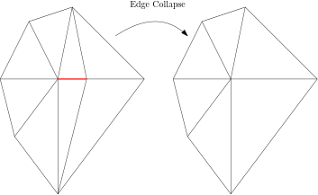
The fundamental operation in Garland and Heckbert’s QEM algorithm is edge collapse, hence its classification as an iterated edge collapse method. As shown in Figure 1, collapsing an edge involves fusing two pendant vertices of an edge. In some cases, we may find it interesting to merge vertices that are not joined by an edge in spite of the possibility of non-manifold (“non-3D-printable”) meshes arising.
Mesh simplification algorithms rooted in iterated edge collapse all boil down to how to decide which edge should be removed at each step. This is facilitated through a cost function, which is an indicator of how much the geometry of the mesh changes when an edge is collapsed. We summarize the algorithm with the following deceptively simple set of instructions.
For each edge, store the cost of a collapse in a priority queue.
Collapse the cheapest edge. That is, we remove the cheapest edge and all adjacent triangles and merge the pendant edges of this edge. The position of the merged vertex may be distinct from those of its ancestors.
Recalculate the cost for all edges altered by the collapse and reorder them within the priority queue.
Repeat from 2 until the stop condition is met.
Quadric error metrics
We now turn to Garland and Heckbert used QEM’s to define a cost function. Suppose we are given a plane in 3D space specified by a normal \(\mathbf{n}\in \mathbf{R}^3\) and the distance of the plane from the origin \(d\in \mathbf{R}\). We can determine the squared distance to a point \(p\) as follows:
where \(A = \mathbf{n} \mathbf{n}^{\mathsf{T}}\) and \(\mathbf{b} = -2d \mathbf{n}\). If we compute $d$ from a point, call it \(\mathbf{p}_0\), in a triangle used to define the plane, then \(d = \mathbf{n}\cdot \mathbf{p}_0\).
So we now have a quadratic function $Q$ called the quadratic error metric represented by the triple $\langle A, \mathbf{b}, d\rangle$. It is also possible to equivalently represent a quadric as a 4×4 matrix via homogeneous coordinates. Measuring the sum of squared distances is straightforward even when we introduce more planes.
In mesh simplification, we compute a QEM for each vertex by summing that for the planes of all incident triangles. We then calculate Q, a QEM for each edge, by summing the QEMs of the endpoints. The cost of collapsing an edge is then \(Q(\mathbf{p})\) where \(\mathbf{p}\) is the position of a collapsed vertex. There are a few ways to place a collapsed vertex. One simple one is to take the position of one of the end-points \(\mathbf{v}_1\) or \(\mathbf{v}_2\) depending on whether \(Q(\mathbf{v}_1) < Q(\mathbf{v}_2)\). We instead optimally place \(\mathbf{p}\). As \(Q\) is a quadratic, its minimum is where \(\nabla Q = 0\), so solving the gradient
Life is not so simple however. \(A\) may not be full rank, e.g. when all the faces contributing to \(Q\) lie on the same plane \(Q = 0\) everywhere on the plane. In such cases we use the singular value decomposition \(A = U \Sigma V^{\mathsf{T}}\) to obtain the pseudoinverse \(A^{\dagger} = V \Sigma^{\dagger} U^{\mathsf{T}}\) with small singular values set to zero to ensure stability.
In any case, once the new vertex position \(\mathbf{p}’\) and its cost \(Q(\mathbf{p}’)\) are found, we store this data in a priority queue. Then we collapse the cheapest edge, place the new merged vertex appropriately, assign a QEM to the merged vertex by summing those of its ancestors, and update and reinsert the QEM’s of all the neighbors of the merged vertex.
Throughout our discussion, notice that there is no condition on the edge loops. Basing the cost function solely on QEM’s does not account for the edge loops, so we must modify it in order to do so. Our idea is to place a frame field on our mesh that indicates preferred directions we would like to collapse an edge along in order to preserve the edge loop structure.
Our contributions
Frame fields
A frame field as introduced by Panozzo et al. is a vector field that assigns to each point on a surface a pair of possibly non-orthogonal, non-unit-length vectors in the tangent plane as well as their opposite vectors. This is a generalization of a cross field, a kind of vector field that has been introduced before frame fields, in the sense that the tangent vectors must be orthogonal and unit-length.
The purpose of both frame and cross fields are to guide automatic quadrangulation methods for triangle meshes, i.e. methods that convert triangle meshes to quadrilateral meshes. Although many field-guided quadrangulation algorithms have been based on fields derived from the surface geometry, in particular its curvature, recent work of Dielen et al. have considered the question of generating fields that produce quadrilateral meshes that mimic what a professional artist would create, e.g. the output meshes have correctly placed edge loops and do not have irregular shading or deformation artifacts. In future work, we hope we can implement this new research to create frame fields that guide our simplification method. Currently, we use a cross field dictated by the principal curvature directions. To describe how our method combines QEMs with alignment to a frame field, we introduce our novel alignment metric.
Alignment Metric
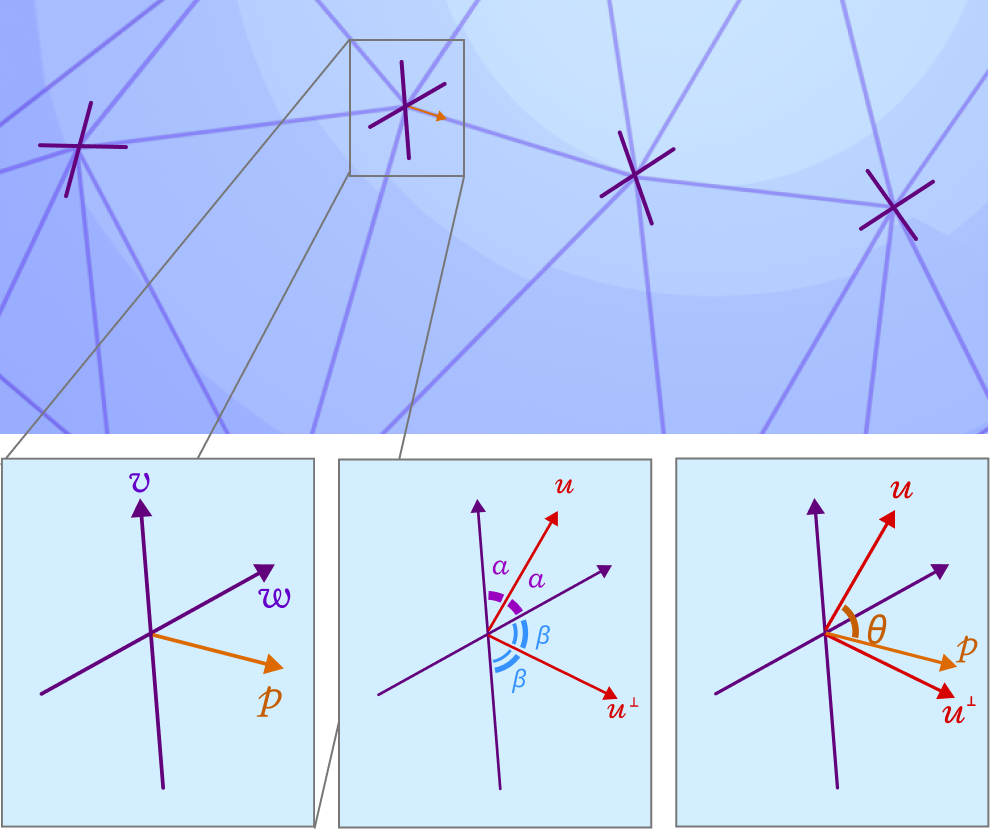
Suppose we are have a point \(x\) on mesh, \(v\) and \(w\) are vectors in the tangent plane that represent the frame field at \(x\), and $p$ is another vector that represents the (orthogonal) projection of an edge emanating from \(x\) that belongs to the mesh. If \(u\) is the bisector of \(\angle vxw\), then, from high school geometry, the orthogonal line \(u^{\perp}\) is also the bisector of \(\angle -vxw\). Intuitively, if \(p\in \operatorname{span} \{u\} \cup \operatorname{span} \{ u^{\perp} \}\), then \(p\) is as “worst” aligned as is possible. So, if \(\theta = \angle pxu\), we would like to find a function \(f\colon [0,\pi]\to [0,1]\) such that \(f(\theta) = 1\) if \(p\in \operatorname{span}{u}\) and \(f(\theta)=0\) if \(p\in \operatorname{span} \{v\}\cup \operatorname{span} \{w\}\), and our cost function for the incremental simplification algorithm should minimize \(f\) among other factors.
So, if \(\alpha = \angle vxu\) and \(\beta = \angle u^{\perp}xw\), then an example alignment function that is differentiable is
With the alignment function in hand, we would like to add it as an additional weight within the cost function of an incremental triangle-based mesh simplification algorithm. We do this simply by multiplying the QEMs by the alignment metric evaluated at the edge that we’re attempting to collapse. For more details, our open source implementation in libigl can be found here. In order to avoid artifacts in the simplified meshes, we have found it helpful to add a small factor, i.e. +1, to the alignment metric.
Results and Future Work
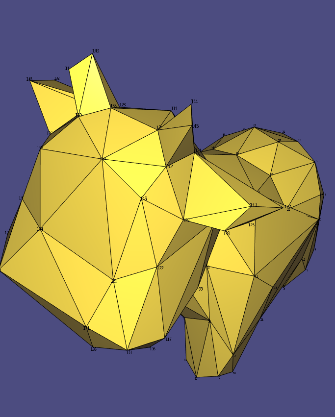
Our results demonstrate that our field-guided, QEM-based mesh simplification method maintains features with high curvature better than Garland and Heckbert’s QEM method. For instance, in the side-by-side comparison below, the ears and horns of Spot in our method (right) have more detail than those in the standard technique of Garland and Heckbert (left).
However, our method in its current iteration still does not preserve edge loop structure and avoid shading irregularities and deformation artifacts to a degree that enable artists to easily edit a simplified mesh. Still, our work is promising in light of the fact that our method simplifies along a frame field not optimized for this purpose, instead prioritizing the surface geometry. We believe that our goal can be achieved by using a frame field generated by the neural method of Dielen et al.
Edge Flips based on Alignment
One idea we still want to build and test out is using edge-flips for getting better edge-loops. Specifically, after each edge-collapse, we look at the one-ring neighborhood of the vertex resulting from the collapsed edge. There, we check all current incident edges and ones that would be incident if an edge-flip is to be applied to one of the vertex’s opposite edges. Finally, the four edges of this set that are best aligned with frame field four directions are selected. Among which, if any of them would result from an edge flip, then we apply it. The animation below shows what the alignment metric of the set of edges with one arbitrary direction looks like.
We initially used a simple dot product for testing alignment, but it seems promising to use the alignment metric discussed earlier and compare the results.
References
Bærentzen, Jakob Andreas, et al. Guide to Computational Geometry Processing. Springer, 2012. DOI.org (Crossref), https://doi.org/10.1007/978-1-4471-4075-7.
Dielen, Alexander, et al. “Learning Direction Fields for Quad Mesh Generation.” Computer Graphics Forum, vol. 40, no. 5, Aug. 2021, pp. 181–91. DOI.org (Crossref), https://doi.org/10.1111/cgf.14366.
Garland, Michael and Paul S. Heckbert. “Surface simplification using quadric error metrics.” Proceedings of the 24th annual conference on Computer graphics and interactive techniques (1997): n. Pag.
Panozzo, Daniele, et al. “Frame Fields: Anisotropic and Non-Orthogonal Cross Fields.” ACM Transactions on Graphics, vol. 33, no. 4, July 2014, p. 134:1-134:11. ACM Digital Library, https://doi.org/10.1145/2601097.2601179.
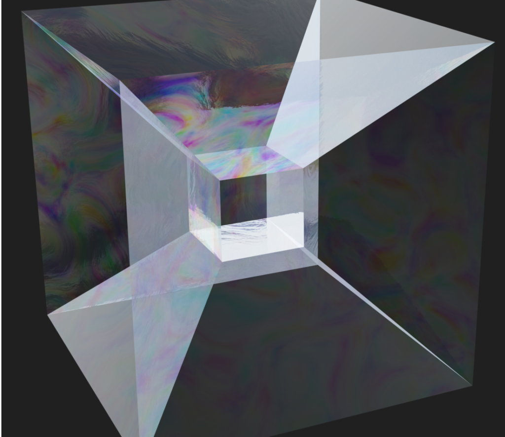
The majority of surfaces in our daily lives are manifold surfaces. Roughly speaking, a manifold surface is one where, if you zoom in close enough at every point, the surface begins to resemble a plane. Most algorithms in computer graphics and digital geometry have historically been tailored for manifold surfaces and fail to preserve or even process non-manifold structures. Non-manifold geometries appear naturally in many settings however. For instance, a dress shirt pocket is sewn onto a sheet of underlying fabric, and these seams are fundamentally non-manifold. Non-manifold surfaces arise in nature in a variety of other settings too, from dislocations in cubic crystals on a molecular level, to the tesseract structures that appear in real world soap films (see Figure 1) [Ishida et al. 2020, Ishida et al. 2017].
Figure 1: Soap film covering the non-manifold minimal surface of a tesseract structure.
The study of soap films connects very closely to a rich vein of study concerning the geometry of minimal surfaces with boundary. The explicit representation of minimal surfaces has a rich history in geometry processing, dating back to the classic paper by Pinkall and Polthier 1993 . Since then, there has been continued study within computer graphics for robust algorithms for computing minimal surfaces, something which is broadly referred to as “Plateau’s Problem”.
Recent work in computer graphics [Wang and Chern 2021] introduced the idea of computing minimal surfaces by solving an “Eulerian” style optimization problem, which they discretize on a grid. In this SGI project, we explored an extension of this idea to the non-manifold setting.
II. Surface Representations
There are multiple ways to digitally represent surfaces, each one with different properties, advantages and disadvantages. Explicit surface representations, such as surface meshes, are easy to model and edit in an intuitive way by artists, but are not very convenient in other settings like constructive solid geometry (CSG). In contrast, implicit surfaces allow to perform morphological operations, and recent advances, such as neural implicits, are also exciting and promising [Xie et al. 2022].
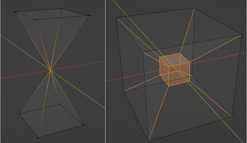
One practical advantage of explicit surface representations like triangle meshes is that they are flexible and intuitive to work with. Triangle meshes are a very natural way to represent manifold surfaces, i.e. surfaces that satisfy the property that the neighborhood of every point is locally similar to the Euclidean plane (or half-plane, in the case of boundaries), and many applications, like 3D printing, require target geometries to be manifold. Triangle meshes can naturally capture non-manifold features as well by including vertices that connect otherwise disjoint triangle fans as in (Figure 2, left) or by edges that are shared by more than two faces (Figure 2, right).
Figure 2: Examples of non-manifold meshes. Non-manifold vertices and edges are highlighted in orange. Left: mesh containing a non-manifold vertex. Right: mesh containing non-manifold edges. Blender highlights faces composed solely by non-manifold edges.
However, in many real world settings, geometric data is not naturally acquired as or represented by a triangle mesh. In applications ranging from medical imaging to constructive solid geometry, the preferred geometric representation is as implicit surfaces.
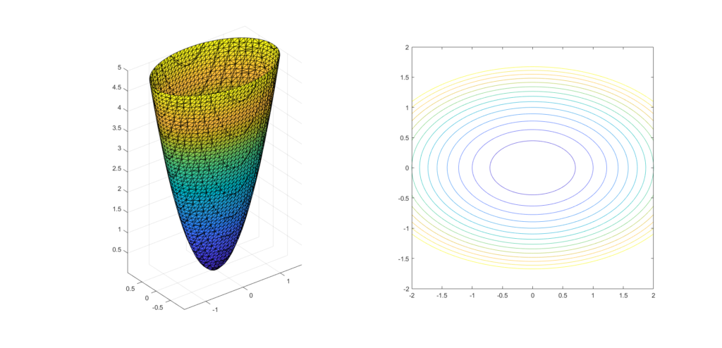
In 2D, implicit surfaces can be described by a function \(f: \mathbb{R}^{2} \rightarrow \mathbb{R}\) that is described by the points \((x, y) \in \mathbb{R}^{2}\) such that \(f(x, y) = c\) for some real value \(c\). By varying the values of \(c\) a set of curves, called level sets, can be used to represent the surface. Figure 3 shows two representations of the same paraboloid, one using an explicit triangle mesh representation (left) and one using level sets of the implicit function (right).
Figure 3: Two distinct representations of the same surface. Left: explicit representation of a hyperboloid using a surface mesh. Right: implicit representation of a hyperboloid using level sets.
While non-manifold features are naturally represented in explicit surface representations, one limitation of implicit surfaces and level sets is that they do not naturally admit a way to represent geometries with non-manifold topology and self-intersections. In this project we focused on studying a way of representing implicit surfaces based on the mathematical machinery of integrable vector fields defined on a background domain.
III. Representing Implicit Surfaces as Integrable Vector Fields
In this project our goal was to explore implicit representations of non-manifold surfaces. To do this, we set out to represent implicit function implicitly, as an integrable vector field.
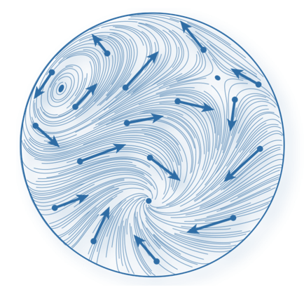
A vector field \(V: \mathbb{R}^{m} \rightarrow \mathbb{R}^{n}\) is a function that corresponds a vector for each point in space. In our case, we are interested in cases where \(m = n = 2\) or \(m = n = 3\); see Figure 4 for an illustration of a vector field defined on a surface. Vector field design and processing is a vast topic, with enough content to fill entire courses on the subject – we refer the interested reader to Goes et al. 2016 and Vaxman et al. 2016 for details.
Figure 4: Vector field defined on a surface. Source: Goes et al. 2016.
One way of thinking of implicit surfaces is as constant valued level sets of some scalar function defined over the entire domain. Our approach was to represent this scalar function as a function of a vector field which we received as an input to our algorithm.
To reconstruct a scalar field from the vector field, it is necessary to integrate the field, which led us into the discussion of integrability of vector fields. A vector field is integrable when it is the gradient of a scalar function. More precisely, the vector field \(V\) is integrable if there is a scalar function \(f\) such that \(V = \nabla f\).
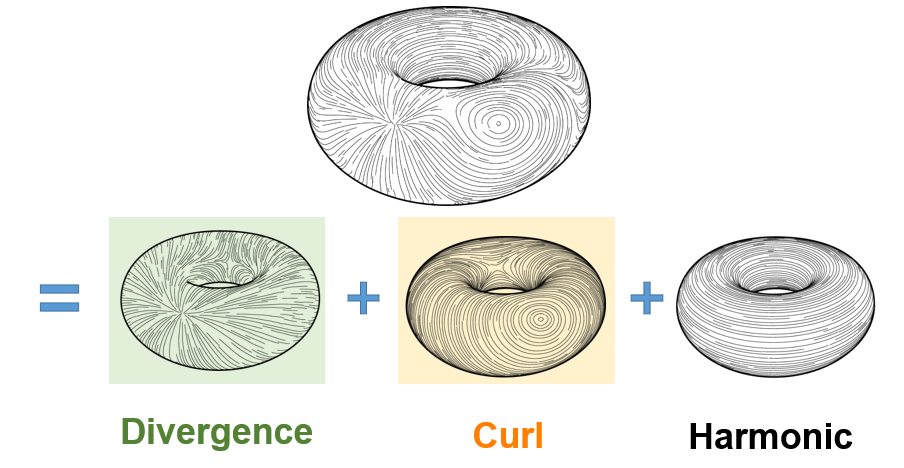
Since it can be arbitrarily hard to find the function \(f\) such that \(V = \nabla f\), or this function may even not exist at all, an equivalent but more convenient condition to check if a vector field is integrable is whether the vector field it is curl-free, that is, if \(\nabla \times V = 0\) for all points in space (Knöppel et al. 2015, Polthier and Preuß 2003). If the vector field is not curl-free, then it is non-integrable, and there is no \(f\) such that \(V = \nabla f\). A possible approach to remove non-integrable features is to apply the Helmholtz-Hodge decomposition, which decomposes the field \(V\) into the sum of three distinct vector fields:
\(\begin{equation} V = F + G + H \end{equation}\)
such that \(F\) is curl-free, \(G\) is divergence-free and \(H\) is a harmonic component. The curl-free \(F\) component is integrable. Figure 5 visualizes this decomposition.
Figure 5: Helmholtz-Hodge decomposition of a vector field defined over a surface. Source: Adapted from Goes et al. 2016.
The non-integrable regions of the vector field correspond to regions where the vector field vanishes or is undefined, also called singularities. For a standard vector field, singular points can be located by checking if the Jacobian is a singular matrix. For implicit non-manifold surfaces, removing the singularities using Helmholtz-Hodge decomposition is not particularly interesting, because the singularities are the cause of the non-manifold features that we want to preserve. At the same time, the singularities prevent the integration of the field, which we wanted to do to reconstruct the levels sets of the implicit function. This dichotomy suggests two different approaches to reconstructing the surface, as described in Section V.
IV. Representing Non-Manifold surfaces as Integrable Frame Fields
Frame Fields or poly-vector fields are generalizations of vector fields which store multiple distinct directions at each point. This terminology was introduced to the graphics literature by Panozzo et. al. 2014, and a technique for generating such integrable fields was presented by Diamanti et. al. 2015.
Animation 1 illustrates one curious phenomenon related to the topology of directional and frame fields. Assume each direction is uniquely labelled (e.g., each different direction is assigned a different color). If you start labelling an arbitrary direction and smoothly circulates around the singularity, trying to consistently label each direction with a unique color, this necessarily causes a mismatch between the initial label and the final label at the starting point. As can be seen in the last frame of the animation, a flow line that was initially assigned a green color was assigned a different color (red) in the last step, characterizing a mismatch between the initial and final label of that flow line. This happens for all the directions.
Animation 1: Failure to uniquely label each flow line direction around a singularity in a directional field. The initial flow line was labelled green. Source: Adapted from Knöppel et al. 2013.
V. Surface Reconstruction
The task can be specifically described as follows: given a frame field defined on a volumetric domain (i.e., a tetrahedral mesh), our goal is to reconstruct a non-manifold surface mesh that represents a non-manifold implicit surface. Two distinct approaches were explored: (i) stream surface tracing based on the alignment of the vector fields and (ii) Poisson surface reconstruction.
V.1. Stream Surface Tracing
The first approach consisted in using stream surfaces to represent the non-manifold surface. Stream surfaces are surfaces whose normal are aligned with one of the three vectors of the frame field. These types of surfaces are usually employed to visualize flows in computational fluid dynamics (Peikert and Sadlo 2009). Many ideas of the algorithm we explored are inspired by Stutz et al. 2022, which further extends the stream surface extraction with an optimization objective to generate multi-laminar structures for topology optimization tasks.
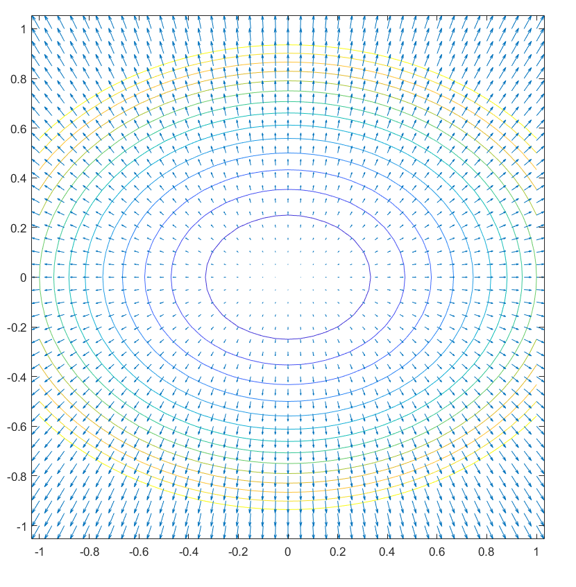
It is known that the gradient \(\nabla f\) of a function \(f\) is perpendicular to the level sets of the function (see Figure 6 for a visual demonstration). Therefore, if we had the gradient of the function, it would be possible to extract a surface by constructing a triangle mesh whose normal vectors of each face are given by the gradient of the function. The main idea of the stream surface tracing is that the input frame field can be used as an approximation of the gradient of the function that we are trying to reconstruct. In other words, the normal vector of the surface is aligned with one of the vectors of the frame field.
Figure 6: the gradient \(\nabla f\) of a function \(f\) is perpendicular to the level sets of \(f\).
Animation 2 displays a step-by-step sequence for the first two tetrahedrons that are visited by the stream surface tracing algorithm, that proceeds as follows:
Choose an initial tetrahedron to start the tracing;
Compute the centroid of the first tetrahedron;
Choose one of the (three) vectors of the frame field as a representative of the normal vector of the surface;
Intersect a plane with the centroid of the tetrahedron such that the previous chosen vector is normal to this plane;
Choose a neighbor tetrahedron that shares a face with the edges that were intersected in the previous step;
For the new tetrahedron, compute the centroid and choose a vector of the frame field (similar to steps 2 and 3);
Project the midpoint of the edge of the previous plane into a line that passes through the centroid of the new tetrahedron.
Intersect a plane with the point computed in the previous step and the new tetrahedron.
Repeat steps 5 through 8 until all tetrahedrons are visited.
After repeating the procedure for all the tetrahedrons in the volumetric domain, a stream surface is extracted that tries to preserve non-manifold features.
Animation 2: Illustration of the main steps of the stream surface algorithm applied to the first two tetrahedra. This procedure is repeated for all tetrahedra in the volumetric domain.
V.1.1 – Results using Vector Fields
Animation 3 demonstrates the stream surface tracing algorithm for a frame field defined on a volumetric domain. In this case, it can be seen that the algorithm extracts a Möbius strip, which is a non-orientable manifold surface.
Animation 3: Stream surface tracing incrementally reconstructing a Möbius strip.
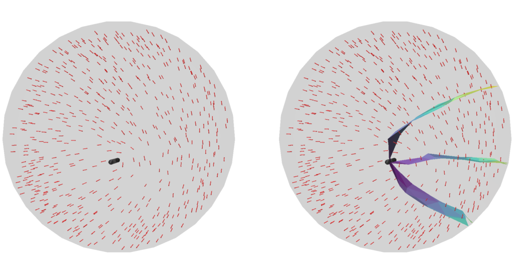
However, the Möbius strip is still a manifold surface and we want to reconstruct non-manifold surfaces. As an example of a surface with non-manifold structures, consider Figure 7. Figure 7, left, shows a frame field and the singularity graph associated with it, while Figure 7, right, presents the surface by the algorithm. The output of the algorithm is a surface mesh containing a non-manifold vertex in the neighborhood of the singular curve, indicating the non-integrability of the field.
Figure 7: Left: frame field and associated singular curve. Right: surface extracted using the surface tracing algorithm. Notice the formation of a T-junction in the neighborhood of the singular curve.
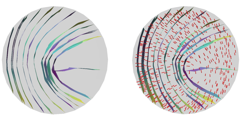
By applying the stream surface tracing algorithm starting from different tetrahedrons, it is possible to trace multiple level sets of the implicit non-manifold surface. Figure 8 displays the result of such procedure, where multiple strips were extracted corresponding to different level sets. Figure 8, right, shows the frame field together with the extracted surfaces: here, it is possible to notice that each vector is approximately normal to the surfaces. This was expected, since the assumption of the algorithm was that the frame field can be used as an approximation of the gradient of the function we want to reconstruct.
Figure 8: Left: reconstructed surfaces for different level sets of the function. Right: surfaces and the corresponding vector field. Notice how the vectors are roughly orthogonal to the level sets, as expected.
V.1.2. Volumetric Frame Fields: Working with Frame Fields in 3D volumes
Implicit functions, as described above, are real-valued functions with infinitely many values. To represent them on a computer, some sort of spatial discretization is necessary. Two common choices are to discretize the space using regular grids or unstructured meshes where each element is a triangle or a tetrahedron. This discretization corresponds to an Eulerian approach: for a fixed discretized domain, the values of the vector fields associated with the implicit functions are observed in fixed locations in space. In this project, tetrahedral meshes are used to discretize the space and fill the volume where the functions are defined.
A tetrahedral mesh is similar to a triangle mesh, but augmented with additional data for each tetrahedron. Formally, a tetrahedral mesh \(\mathcal{M}\) is defined by a set \({\mathcal{V}, \mathcal{E}, \mathcal{F}, \mathcal{T}}\) of vertices, edges, faces and tetrahedrons, respectively. Each tetrahedron is composed of 4 vertices, 6 edges and 4 faces. The edges and faces of one tetrahedron may be shared with adjacent tetrahedrons, which allow to traverse the mesh. More importantly, this allows to define the vector field using the tetrahedral mesh as a background domain to discretize the function over this volumetric space.
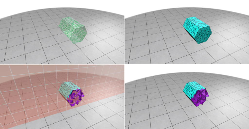
As input, we start with a boundary mesh enclosing a volume (Figure 9, top left). Bear in mind that this boundary mesh does not fill the space, but only specifies the boundary of a region of interest. We can fill the volume using a tetrahedral mesh (Figure 9, top right). This tetrahedralization can be done using Fast Tetrahedral Meshing in the Wild, for instance. It is important to notice that, in contrast to a surface polygon mesh, a tetrahedral mesh is a volume mesh in the sense that it fills the volume enclosed by it. If we slice the tetrahedral mesh with a plane (Figure 9, bottom left and bottom right), we can see that the interior of the tetrahedral mesh is not empty (as would be the case for a surface mesh) and that the interior volume is fully filled. In Figure 9, the interior faces of the tetrahedrons were colored in purple while the boundary faces were colored in cyan.
Figure 9: Tetrahedralization of a boundary domain. Starting with a boundary domain bounded by a surface mesh (top left), the domain is discretized using tetrahedrons (top right). Unlike a surface mesh, a volumetric mesh fills the interior space of the volume it discretizes (bottom row).
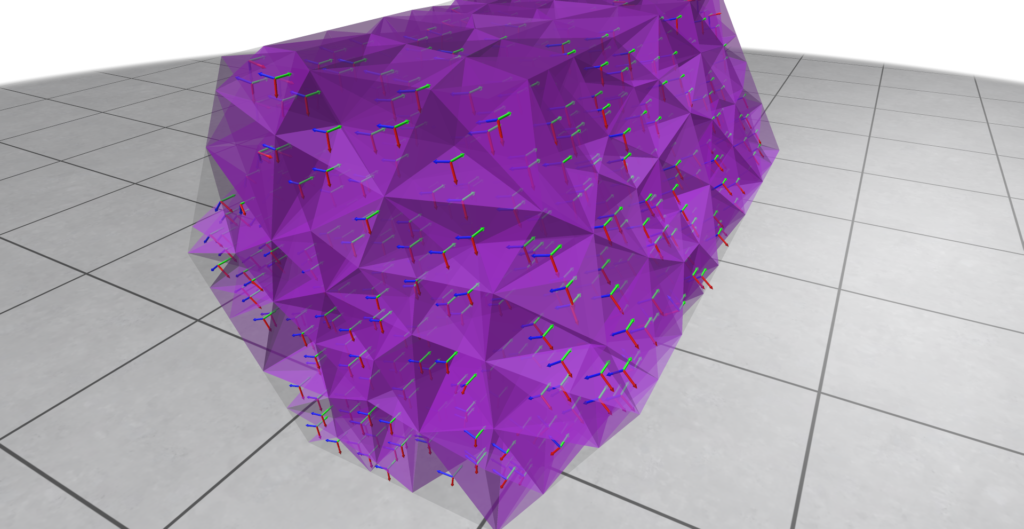
Three distinct vector fields \(U, V, W\) constitute a volumetric frame field if they form an orthonormal basis at each point in space. As mentioned, we work with frame fields defined on a volumetric domain as a representation of the implicit non-manifold surface. Each tetrahedron will be associated with three orthogonal vectors, as shown in Figure 10.
Figure 10: Sample of data used to represent a non-manifold implicit surface. The domain was discretized using tetrahedral meshes (purple). Each tetrahedron is associated with three orthogonal vectors, that constitute a volumetric frame field.
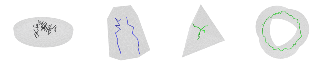
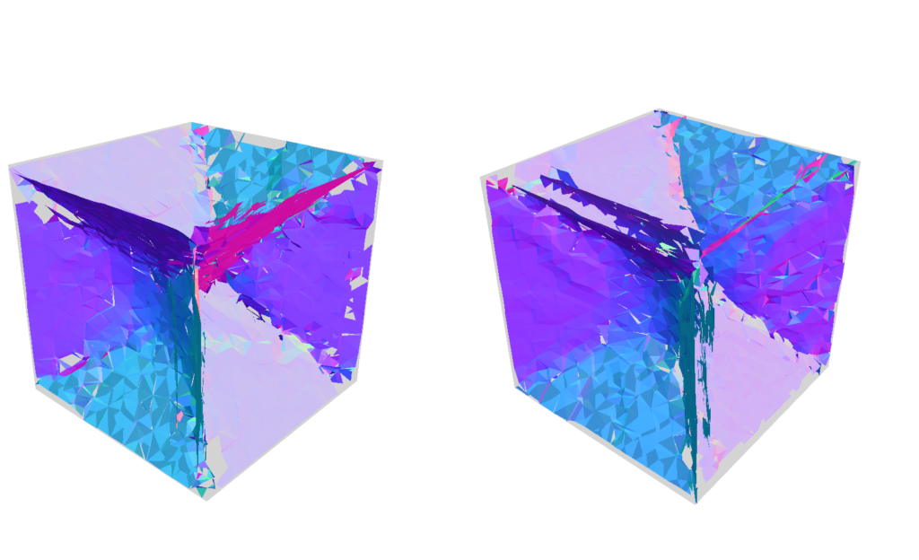
The previous idea of labelling directions around a point can be useful to detect singularities in our frame fields. The same idea can be extended to volumetric frame fields, where singularities create singular curves on the volumetric domain. These curves are denominated as singularity graphs. Figure 11 shows the singularity graphs for some frame fields. See Nieser et al. 2011 for details. Identifying the singular curves on the frame fields is equivalent to identifying its non-integrable regions.
Figure 11: Singularity graphs of the volumetric frame fields.
V.1.3. Results using Volumetric Frame Fields
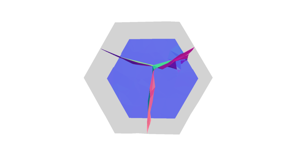
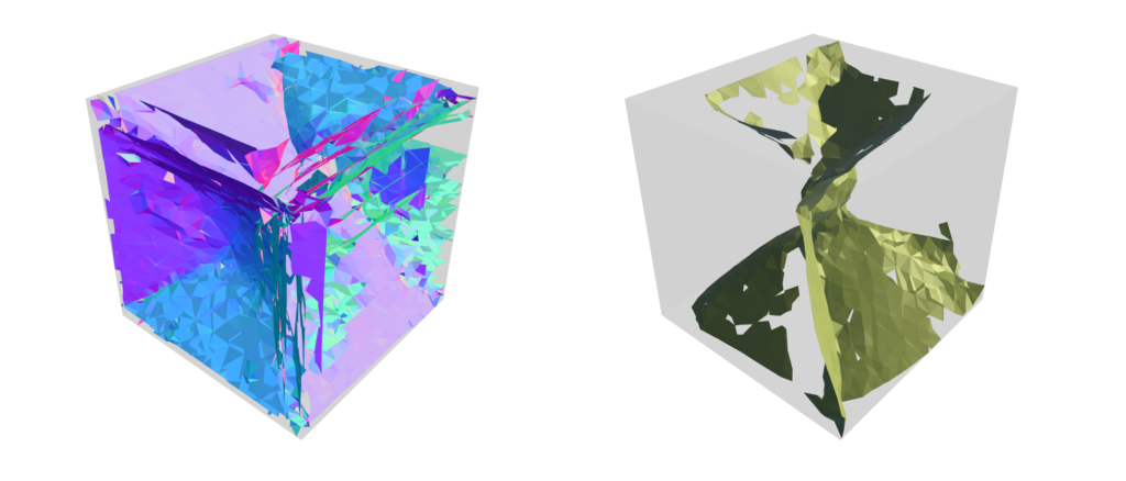
Another example is provided in Figure 12, where the volumetric frame field is defined on a hexagonal boundary mesh. The output presents a non-manifold junction through a non-manifold vertex.
Figure 12: reconstructed surface for a hexagonal boundary mesh.
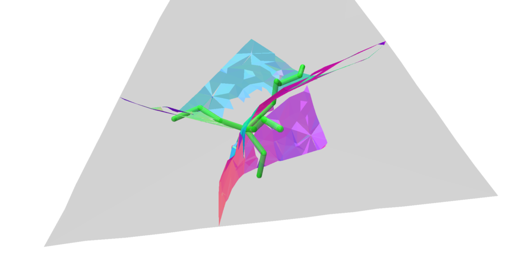
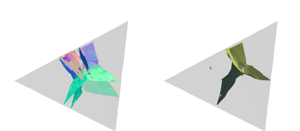
As a harder test case, it can be seen in Figure 13 that the resulting surface extracted by the algorithm is not a perfectly closed mesh. While the surface tries to follow the singularity graph (in green), it fails to self-intersect in some regions, creating undesirable gaps.
Figure 13: reconstructed surface for a tetrahedral boundary mesh and the singularity graph (in green) associated with the volumetric frame field. The surface has an overall structure that resembles the junction present in the singularity graph, but in this case the algorithm wasn’t able to extract a mesh without holes.
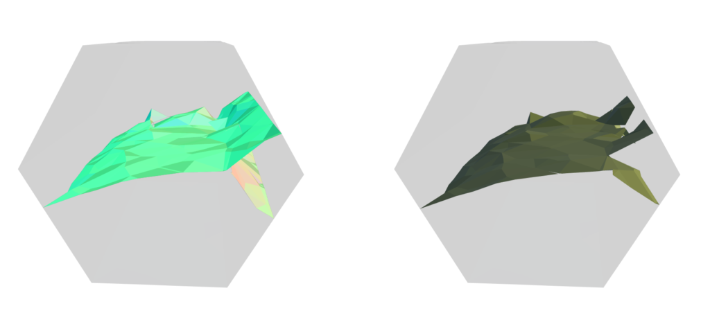
Finally, we tested the algorithm to reconstruct the non-manifold minimal tesseract, presented in Figure 1. Two points of view of the output are presented in Figure 14. While the traced mesh has a structure similar to the desired surface, the result could still be further improved. The mesh presents cracks in the surface and some almost disconnected regions. We applied hole filling algorithms, such as those provided by MeshLab, as an attempt to fix the issue, but they weren’t capable of closing the holes for any combination of parameters tested.
Figure 14: reconstructed surface for the non-manifold minimal surface tesseract. The reconstruction preserves the overall structure of the desired surface. However, the algorithm fails to create a surface without holes and produces some regions that are mostly disconnected from the surface.
V.2. Poisson Surface Reconstruction
The second approach consisted in investigating the classic Poisson Surface Reconstruction algorithm by Kazhdan et al. 2006 for our task. Specifically, our goal was to evaluate whether the non-manifold features were preserved using this approach and, if not, where exactly it fails.
Given a differentiable implicit function \(f\), we can compute its gradient vector field \(G = \nabla f\). This can be done either analytically, if there is a closed-formula for \(f\), or computationally, using finite-element methods or discrete exterior calculus. Conversely, given a gradient vector field \(G\), we can integrate \(G\) to compute the implicit function \(f\) that generates the starting vector field.
Note that since it was assumed that \(G\) is a gradient vector field, and not an arbitrary vector field, this means that \(G\) is integrable. If this is the case, we know that a function \(f\) whose gradient vector field is \(G\) exists; we just need to find it. However, in practice, the input of the algorithm may be a vector field \(V\) which is not exactly integrable due to noise or sampling artifacts. How can \(f\) be computed in all these cases?
One core idea of the Poisson Surface Reconstruction algorithm consists in reconstructing \(f\) using a least-squares optimization formulation:
For a perfectly integrable vector field (i.e., a gradient vector field), it would theoretically be possible to compute \(\tilde{f} = f\) such that \(\nabla \tilde{f} = V\) and reconstruct \(f\) exactly. The advantage of this formulation is that even in cases where the vector field \(V\) is not exactly integrable, it will reconstruct the best approximation of \(f\) by minimizing the least-squares error.
In the case of our frame fields representing non-manifold surfaces, the existence of singularities in the field means that it will necessarily be non-integrable. It is expected that the equality \(\nabla \tilde{f} = V\) fails precisely in the regions containing singular points, but we wanted to evaluate the performance of a classic algorithm on our data.
V.2.1 – Results using Volumetric Frame Fields
Figure 15 and Figure 16 present comparisons between the surface extracted by Stream Surface Tracing and Poisson Surface Reconstruction algorithm for two different inputs. While for the hexagonal boundary mesh (Figure 15) both algorithms have a similar output, for the tetrahedral boundary mesh (Figure 16) Poisson Surface Reconstruction generates a surface closer to the desired non-manifold junction.
Figure 15: Comparison between the Stream Surface Tracing algorithm (left) and the Poisson Surface Reconstruction (right) for the volumetric frame field with hexagonal boundary mesh.
Figure 16: Comparison between the Stream Surface Tracing algorithm (left) and the Poisson Surface Reconstruction (right) for the volumetric frame field with tetrahedral boundary mesh. In this case, Poisson Surface Reconstruction extracts a surface that is closer to the desired junction in comparison to the Stream Surface Tracing.
Remarkably, the Poisson Surface Reconstruction fails badly for the non-manifold tesseract, as shown in Figure 17. While the Stream Surface Tracing doesn’t extract a perfect surface reconstruction (Figure 17, left), it is much closer to the tesseract than the surface reconstructed by the Poisson Surface Reconstruction (Figure 17, right).
Figure 17: Comparison between the Stream Surface Tracing algorithm (left) and the Poisson Surface Reconstruction (right) for the volumetric frame field defined for the tesseract structure. In this case, Poisson Surface Reconstruction drastically fails to preserve the non-manifold structure of the target surface.
VI. Conclusions and Future Work
In this project we explored multiple surface reconstruction algorithms that could possibly preserve non-manifold structures from frame fields defined on tetrahedral domains. While the algorithms could extract surfaces that present the overall structure desired, for many inputs the mesh displayed artifacts such as cracks or components that aren’t completely connected, such as non-manifold vertices where a non-manifold edge was expected. As future work, we consider using the singularity graph to guide the tracing as an attempt to close the holes in the mesh. Another possible direction would be to explore the usage of the singularity graph in the optimization process used in the Poisson Surface Reconstruction algorithm.
I would like to thank Josh Vekhter, Nicole Feng and Marco Ravelo for the mentoring and patience to guide me through the rich and beautiful theory of frame fields. Furthermore, I would like to thank Justin Solomon for the hard work on organizing SGI and baking beautiful singular pies.
Nieser, Matthias, Ulrich Reitebuch, and Konrad Polthier. “Cubecover–parameterization of 3d volumes.” Computer graphics forum. Vol. 30. No. 5. Oxford, UK: Blackwell Publishing Ltd, 2011.
Kazhdan, Michael, Matthew Bolitho, and Hugues Hoppe. “Poisson surface reconstruction.” Proceedings of the fourth Eurographics symposium on Geometry processing. Vol. 7. 2006.

