Fellows: Gizem Altintas, Ikaro Costa, Emi Neuwalder, Kyle Onghai, and Hossam Saeed Volunteers: Shaimaa Monem and Andrew Rodriguez Mentor: Frank Yang
Introduction
In geometry processing, mesh simplification refers to a class of algorithms that convert a given polygonal mesh to a new mesh with fewer faces. Typically, the mesh is simplified in a way that optimizes the preservation of specific, user-defined properties like distortion (Hausdorff distance, normals) or appearance (colors, features).
One application of mesh simplification is adapting high-detail art assets for real-time rendering. Unfortunately, when applying common mesh decimation techniques based on iterated local edge collapse, the resulting mesh can be difficult to edit; local edge collapse and edge flip techniques often do not preserve edge loops or have irregular shading and deformation artifacts.
On the other hand, quad mesh simplification methods like polychord collapse can retain more of the edge loop structure of the original mesh at the cost of more complexity. For example, polychord collapse uses non-local operations on sequences of quads (polychords), and quad remeshing even requires global optimization and reconstruction.
Is there a simpler way that allows us to preserve these edge loops throughout simplification while limiting ourselves to local operations, i.e. edge collapses, flips, and regularization? The original quad mesh might provide a starting point as it seems to define a frame field at most points on the mesh that we can use to perhaps guide our local operations.
The potential benefit of this is we can obtain nicely tessellated quad meshes from either quad meshes or even a not-so-nice triangle mesh without having to resort to more complex techniques such as quad polychord collapse or quad remeshing.
Triangle mesh simplification
The first question one might ask is why do the standard triangular decimation techniques often fail to retain edge loops. We would retort, “Why should they?” There is no mechanism that would coerce standard triangular decimation techniques to preserve edge loops. To convince you of this, we will delve into how the quadric error metric (QEM) mesh simplification method of Garland and Heckbert, one of the most well-known triangular mesh simplification algorithms and the one upon which we have built our own, works.
The fundamental operation in Garland and Heckbert’s QEM algorithm is edge collapse, hence its classification as an iterated edge collapse method. As shown in Figure 1, collapsing an edge involves fusing two pendant vertices of an edge. In some cases, we may find it interesting to merge vertices that are not joined by an edge in spite of the possibility of non-manifold (“non-3D-printable”) meshes arising.
Mesh simplification algorithms rooted in iterated edge collapse all boil down to how to decide which edge should be removed at each step. This is facilitated through a cost function, which is an indicator of how much the geometry of the mesh changes when an edge is collapsed. We summarize the algorithm with the following deceptively simple set of instructions.
For each edge, store the cost of a collapse in a priority queue.
Collapse the cheapest edge. That is, we remove the cheapest edge and all adjacent triangles and merge the pendant edges of this edge. The position of the merged vertex may be distinct from those of its ancestors.
Recalculate the cost for all edges altered by the collapse and reorder them within the priority queue.
Repeat from 2 until the stop condition is met.
Quadric error metrics
We now turn to Garland and Heckbert used QEM’s to define a cost function. Suppose we are given a plane in 3D space specified by a normal \(\mathbf{n}\in \mathbf{R}^3\) and the distance of the plane from the origin \(d\in \mathbf{R}\). We can determine the squared distance to a point \(p\) as follows:
where \(A = \mathbf{n} \mathbf{n}^{\mathsf{T}}\) and \(\mathbf{b} = -2d \mathbf{n}\). If we compute $d$ from a point, call it \(\mathbf{p}_0\), in a triangle used to define the plane, then \(d = \mathbf{n}\cdot \mathbf{p}_0\).
So we now have a quadratic function $Q$ called the quadratic error metric represented by the triple $\langle A, \mathbf{b}, d\rangle$. It is also possible to equivalently represent a quadric as a 4×4 matrix via homogeneous coordinates. Measuring the sum of squared distances is straightforward even when we introduce more planes.
In mesh simplification, we compute a QEM for each vertex by summing that for the planes of all incident triangles. We then calculate Q, a QEM for each edge, by summing the QEMs of the endpoints. The cost of collapsing an edge is then \(Q(\mathbf{p})\) where \(\mathbf{p}\) is the position of a collapsed vertex. There are a few ways to place a collapsed vertex. One simple one is to take the position of one of the end-points \(\mathbf{v}_1\) or \(\mathbf{v}_2\) depending on whether \(Q(\mathbf{v}_1) < Q(\mathbf{v}_2)\). We instead optimally place \(\mathbf{p}\). As \(Q\) is a quadratic, its minimum is where \(\nabla Q = 0\), so solving the gradient
Life is not so simple however. \(A\) may not be full rank, e.g. when all the faces contributing to \(Q\) lie on the same plane \(Q = 0\) everywhere on the plane. In such cases we use the singular value decomposition \(A = U \Sigma V^{\mathsf{T}}\) to obtain the pseudoinverse \(A^{\dagger} = V \Sigma^{\dagger} U^{\mathsf{T}}\) with small singular values set to zero to ensure stability.
In any case, once the new vertex position \(\mathbf{p}’\) and its cost \(Q(\mathbf{p}’)\) are found, we store this data in a priority queue. Then we collapse the cheapest edge, place the new merged vertex appropriately, assign a QEM to the merged vertex by summing those of its ancestors, and update and reinsert the QEM’s of all the neighbors of the merged vertex.
Throughout our discussion, notice that there is no condition on the edge loops. Basing the cost function solely on QEM’s does not account for the edge loops, so we must modify it in order to do so. Our idea is to place a frame field on our mesh that indicates preferred directions we would like to collapse an edge along in order to preserve the edge loop structure.
Our contributions
Frame fields
A frame field as introduced by Panozzo et al. is a vector field that assigns to each point on a surface a pair of possibly non-orthogonal, non-unit-length vectors in the tangent plane as well as their opposite vectors. This is a generalization of a cross field, a kind of vector field that has been introduced before frame fields, in the sense that the tangent vectors must be orthogonal and unit-length.
The purpose of both frame and cross fields are to guide automatic quadrangulation methods for triangle meshes, i.e. methods that convert triangle meshes to quadrilateral meshes. Although many field-guided quadrangulation algorithms have been based on fields derived from the surface geometry, in particular its curvature, recent work of Dielen et al. have considered the question of generating fields that produce quadrilateral meshes that mimic what a professional artist would create, e.g. the output meshes have correctly placed edge loops and do not have irregular shading or deformation artifacts. In future work, we hope we can implement this new research to create frame fields that guide our simplification method. Currently, we use a cross field dictated by the principal curvature directions. To describe how our method combines QEMs with alignment to a frame field, we introduce our novel alignment metric.
Alignment Metric
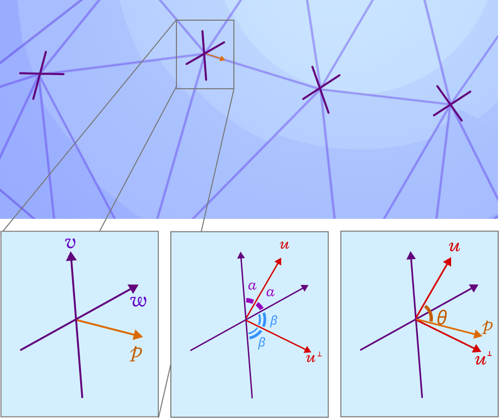
Suppose we are have a point \(x\) on mesh, \(v\) and \(w\) are vectors in the tangent plane that represent the frame field at \(x\), and $p$ is another vector that represents the (orthogonal) projection of an edge emanating from \(x\) that belongs to the mesh. If \(u\) is the bisector of \(\angle vxw\), then, from high school geometry, the orthogonal line \(u^{\perp}\) is also the bisector of \(\angle -vxw\). Intuitively, if \(p\in \operatorname{span} \{u\} \cup \operatorname{span} \{ u^{\perp} \}\), then \(p\) is as “worst” aligned as is possible. So, if \(\theta = \angle pxu\), we would like to find a function \(f\colon [0,\pi]\to [0,1]\) such that \(f(\theta) = 1\) if \(p\in \operatorname{span}{u}\) and \(f(\theta)=0\) if \(p\in \operatorname{span} \{v\}\cup \operatorname{span} \{w\}\), and our cost function for the incremental simplification algorithm should minimize \(f\) among other factors.
So, if \(\alpha = \angle vxu\) and \(\beta = \angle u^{\perp}xw\), then an example alignment function that is differentiable is
With the alignment function in hand, we would like to add it as an additional weight within the cost function of an incremental triangle-based mesh simplification algorithm. We do this simply by multiplying the QEMs by the alignment metric evaluated at the edge that we’re attempting to collapse. For more details, our open source implementation in libigl can be found here. In order to avoid artifacts in the simplified meshes, we have found it helpful to add a small factor, i.e. +1, to the alignment metric.
Results and Future Work
Our results demonstrate that our field-guided, QEM-based mesh simplification method maintains features with high curvature better than Garland and Heckbert’s QEM method. For instance, in the side-by-side comparison below, the ears and horns of Spot in our method (right) have more detail than those in the standard technique of Garland and Heckbert (left).
However, our method in its current iteration still does not preserve edge loop structure and avoid shading irregularities and deformation artifacts to a degree that enable artists to easily edit a simplified mesh. Still, our work is promising in light of the fact that our method simplifies along a frame field not optimized for this purpose, instead prioritizing the surface geometry. We believe that our goal can be achieved by using a frame field generated by the neural method of Dielen et al.
Edge Flips based on Alignment
One idea we still want to build and test out is using edge-flips for getting better edge-loops. Specifically, after each edge-collapse, we look at the one-ring neighborhood of the vertex resulting from the collapsed edge. There, we check all current incident edges and ones that would be incident if an edge-flip is to be applied to one of the vertex’s opposite edges. Finally, the four edges of this set that are best aligned with frame field four directions are selected. Among which, if any of them would result from an edge flip, then we apply it. The animation below shows what the alignment metric of the set of edges with one arbitrary direction looks like.
We initially used a simple dot product for testing alignment, but it seems promising to use the alignment metric discussed earlier and compare the results.
References
Bærentzen, Jakob Andreas, et al. Guide to Computational Geometry Processing. Springer, 2012. DOI.org (Crossref), https://doi.org/10.1007/978-1-4471-4075-7.
Dielen, Alexander, et al. “Learning Direction Fields for Quad Mesh Generation.” Computer Graphics Forum, vol. 40, no. 5, Aug. 2021, pp. 181–91. DOI.org (Crossref), https://doi.org/10.1111/cgf.14366.
Garland, Michael and Paul S. Heckbert. “Surface simplification using quadric error metrics.” Proceedings of the 24th annual conference on Computer graphics and interactive techniques (1997): n. Pag.
Panozzo, Daniele, et al. “Frame Fields: Anisotropic and Non-Orthogonal Cross Fields.” ACM Transactions on Graphics, vol. 33, no. 4, July 2014, p. 134:1-134:11. ACM Digital Library, https://doi.org/10.1145/2601097.2601179.
By SGI Fellows: Anna Cole, Francisco Unai Caja López, Matheus da Silva Araujo, Hossam Mohamed Saeed
I. Introduction
In this project, mentored by Professor Paul Kry, we are exploring properties and applications of multiresolution surface representations: surface meshes with different complexities and details that represent the same underlying surface.
Frequently, the digital representation of intricate and detailed surfaces requires huge triangle meshes. For instance, the digital scan of Michelangelo’s statue of David [9] contains over 1 billion polygon faces and requires 32 GB of memory. The high level of complexity makes it costly to store and render the surface. Furthermore, applying standard geometry processing algorithms on such complex meshes requires huge computational resources. An alternative consists in representing the underlying surface using hierarchy of meshes, also known as multiresolution representations [2]. Each successive level of the hierarchy uses a mesh with lower geometric complexity while representing the same smooth surface. A hierarchy of meshes allows to represent surfaces at different resolutions, which is critical to handle complex geometric models. This form of representation provides efficiency and scalability for rendering and processing of complex surfaces, because the level of detail of the surface can be adjusted based on the hardware available. Figure 1 shows one example of a hierarchy of meshes. In this project we explore the construction of hierarchical representations of surface meshes combined with correspondences between different levels of the hierarchy.
Figure 1: a hierarchy of meshes built using mesh simplification.
One critical point of this construction is a mapping between meshes at different levels. Liu et al. 2020 [7] proposes a bijective map, named successive self-parameterization, that allows to correspond coarse and fine meshes on the multiresolution hierarchy. To build this mapping, successive self-parameterization requires a (i) mesh simplification algorithm to build the hierarchy of meshes and (ii) a conformal parameterization to map meshes on successive refinement levels to a common space. Our goal for this project is to investigate different applications of this mapping. In the next sections, we detail the algorithms to construct the hierarchy and the successive self-parameterization.
II. Mesh simplification
II.1. Mesh simplification using quadric error
The mesh simplification algorithm studied was introduced in Garland and Heckbert 1997 [6] and is quite straightforward: it consists in collapsing various edges of the mesh sequentially. Specifically, in each iteration, two neighboring vertices \(v_i\) and \(v_j\) will be chosen and replaced by a single vertex \(\overline{v}\). The new vertex \(\overline{v}\) will inherit all neighbors of \(v_i\) and \(v_j\). In Animation 1 it is possible to see the possible result of two edge collapses in a triangle mesh.
Animation 1: consecutive edge collapses in a triangle mesh.
Suppose we have decided to collapse edge \((v_i,v_j)\). Then, \(\overline{v}\) is found as the solution of a minimization problem. For each vertex \(v_i\) we define a matrix \(Q_i\) so that \(v^TQ_iv\), with \(v=[v_x, v_y, v_z, 1]\), gives a measure of how far \(v\) is from \(v_i\). We choose \(\overline{v}\) minimizing \(v^T(Q_i+Q_j)v\). As for the choice of the \(Q\) matrices, we consider:
To each vertex \(v_i\) we associate the set of planes corresponding to faces that contain \(v_i\) and denote it \(\mathcal{P}(v_i)\).
For each face of the mesh we consider \(p=[a,b,c,d]^T\) such that \(v^Tp=0\) is the equation of the plane and \(a^2+b^2+c^2=1\). This allows us to compute the distance from a point \(v=[v_x,v_y,v_z,1]\) to the plane as \(\vert v^Tp \vert\).
Then, the sum of the squared distances from \(v\) to each plane in \(\mathcal{P}(v_i)\) would be
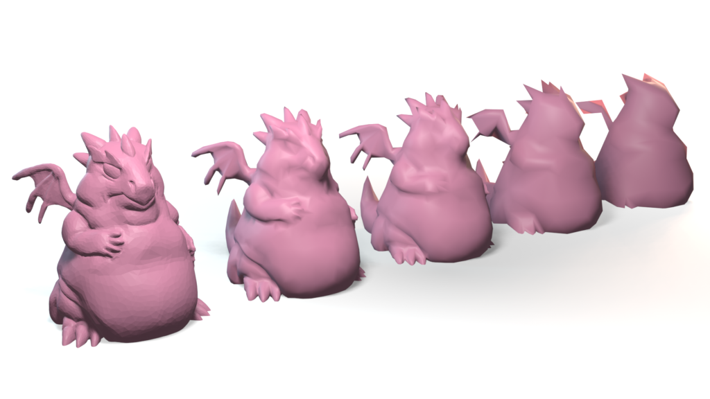
Finally, we decide which edge to collapse by choosing \((v_i,v_j)\) minimizing the error \(\overline{v}^T(Q_i+Q_j)\overline{v}\). For the following iterations, \(\overline{v}\) is assigned the matrix \(Q_i+Q_j\). Animations 2 and 3 illustrates the process of mesh simplification using quadric error.
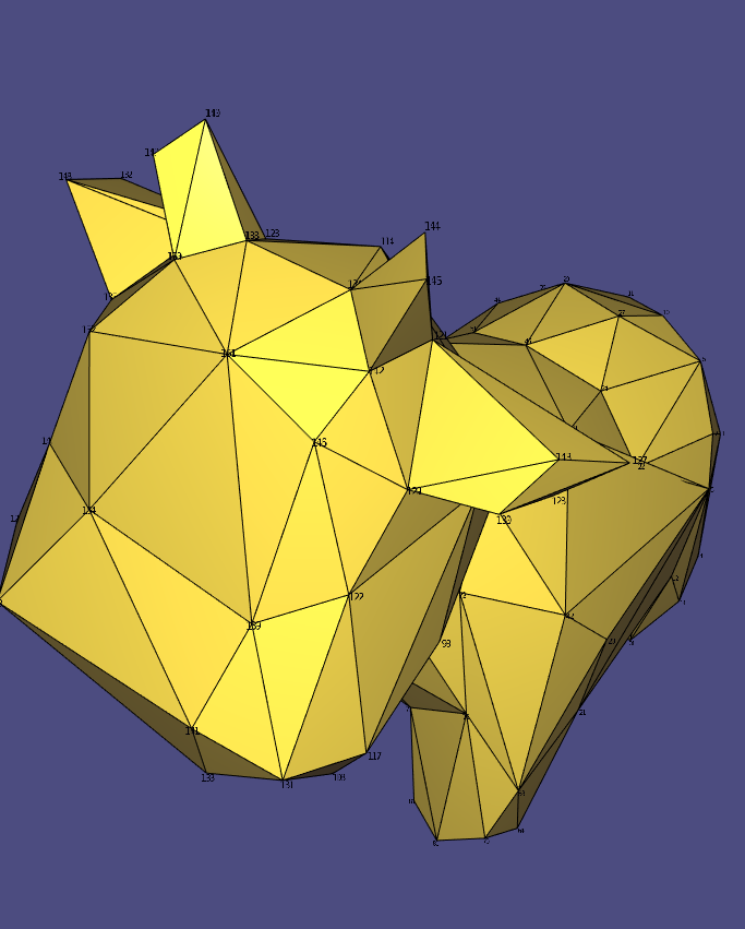
Animation 2: mesh simplification of Spot.
Animation 3: mesh simplification of Fennec Fox.
The algorithm can also run on meshes with boundaries. In Animation 4 we chose not to collapse boundary edges, which allows the boundaries to be preserved.
Animation 4: simplification of a mesh with boundaries. In this case, the boundary of the mesh is preserved.
II.2. Manifoldness and edge collapse validation
There are a variety of issues that can occur if we collapse each edge only based on the error quadrics \(Q_i+Q_j\). This is because the error quadric is only concerned with the geometry of the meshes but not the topology. So we needed to implement some connectivity checks to make sure the edge collapse wouldn’t result in a non-manifold case or change the topology of the mesh.
This can be visualized in Animation 5, where collapsing an interior edge consisting of two boundary vertices can create a non-manifold edge (or vertex). Another problematic case is collapsing an edge with its two vertices sharing more than two neighboring vertices, which would break manifoldness. We followed the criteria described in Liu et al. 2020 [7] and Hoppe el al. 1993 [5] to guarantee an manifold input mesh stays manifold after each collapse. Also, we added the condition where we compute the Euler characteristic \(\chi(M)\) before and after the collapse and if there is a change, we revert back and choose a different edge. In case all remaining edges are not valid for the collapse operation, we simply stop the collapsing process and move on to the next step.
Animation 5: examples of valid edge collapses (left and center figures, in blue) and an example of an edge collapse that generates non-manifold elements (right figure, in orange).
III. Mesh parameterization
Mesh parameterization deals with the problem of mapping a surface to the plane. In our case, the surface is represented by a triangle mesh. This means that for every vertex of the triangle mesh we find corresponding coordinates on the 2D plane. More precisely, given a triangle mesh \(\mathcal{M}\), with a set of vertices \(\mathcal{V}\) and a set of triangles \(\mathcal{T}\), the mesh parameterization problem is concerned with finding a map \(f: \mathcal{V} \rightarrow \Omega \subset \mathbb{R}^{2}\). The effect of this mapping can be seen in Animation 6, where one 3D mesh is flattened to the 2D plane.
Animation 6: a triangle mesh embedded in \(\mathbb{R}^{3}\) is flattened to the 2D plane using a mesh parameterization algorithm.
This mapping enables all sorts of interesting applications. The most famous one is texture mapping: how to specify texture coordinates for each vertex of a triangle mesh such that you can map a region of an image to the mesh? Other applications include conversion of triangle meshes into parametric surfaces [11] e.g., T-Splines or NURBS and computational fabrication [12]. In this section we won’t give all the details about this field, but rather will focus on the aspects relevant to build mappings between meshes of different refinement levels on the hierarchical surface representation. We refer the interested reader to Hormann et al. 2007 [10] for an extensive treatment.
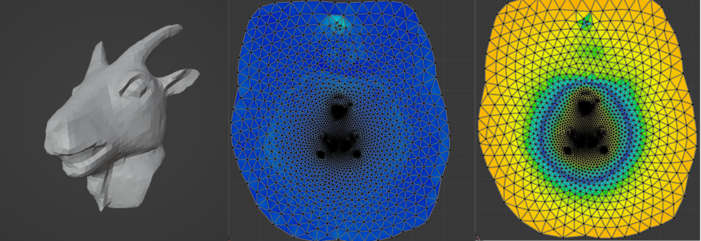
There are many different possibilities to define the mapping from the surface to the plane. However, this mapping usually introduces undesirable distortions. Depending on the construction used, the map may preserve areas, but not angles or orientations; conversely, it may preserve angles but not areas and lengths. This can be seen in Figure 2, where we can visualize angles and area distortions in the parameterized mesh.
Figure 2 : given a triangle mesh (left), we can map it to the 2D plane (center and right). This mapping can introduce angle distortions (center) and area distortions (right).
To create maps between meshes of different levels, Liu et al. 2020 [7] uses conformal mappings, which are maps that preserve angles. Conformal mappings are efficient to compute and provide theoretical guarantees, making it a common choice for many geometry processing tasks.
A conformal map is characterized by the Cauchy-Riemann equations:
Conformal mappings also have a strong connection with complex analysis, which leads to an alternative but equivalent formulation of the problem.
For arbitrary triangle meshes it is impossible to find an exact conformal mapping; only developable meshes (i.e., meshes with zero Gaussian curvature at every point) can be conformally parameterized. In most cases, this restriction is too severe. To work around this, it is possible to build a conformal mapping satisfying the previous equations as close as possible. In other words, we can associate it with an energy function to find the mapping that better approximates a conformal mapping using a least squares formulation:
where \(S\) is the smooth surface represented by a triangle mesh \(\mathcal{M}\).
On a triangle mesh, the functions \(u(x, y), v(x,y)\) can be written with respect to the local orthonormal coordinate system of the triangle. Since the triangle mesh is a piecewise linear surface, the gradient of a function defined over the mesh is constant with respect to each triangle. This makes it possible to find the mapping that better approximates the Cauchy-Riemann equations for each triangle of the mesh. Hence, in this discrete setting, the previous equation can be rewritten as follows
where \(A_{t}\) denotes the area of each triangle with vertices represented by \((i, j, k)\). The solution of the discrete conformal energy described above are the coordinates \((u, v)\) in the 2D plane for each vertex of each triangle \(t\) in the set of triangles \(\mathcal{T}\) of the mesh \(\mathcal{M}\). More details can be found in Lévy et al. 2002 [4] and Desbrun et al. 2002 [13].
However, the trivial solution for this equation would be to set all coordinates \((u, v)\) to the same point and the energy would be minimized, which is not what we want. Therefore, to prevent this case, it is necessary to fix or pin two arbitrary vertices to arbitrary positions in the plane. This restriction generates a least squares problem with a unique solution. The choice of the vertices to be fixed is arbitrary but can have impact on the quality and numerical stability of the parameterization. For instance, there can be arbitrary area distortions depending on the vertices that are fixed. To prevent the problem of the trivial solution while preserving numerical stability, an alternative strategy is proposed by Mullen et al. 2008 [3] in which the system is reformulated to an equivalent eigendecomposition problem which avoid the need to pin any vertex.
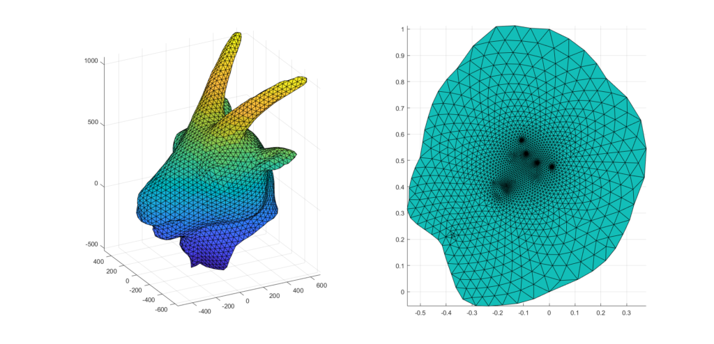
Figure 3 illustrates the least squares conformal mapping obtained for a triangle mesh with boundaries. Notice that the map obtained doesn’t necessarily preserve areas and lengths. Furthermore, as can be seen in the right plot of the figure, lots of details are grouped around tiny regions in the interior of the parameterized mesh.
Figure 3: a triangle mesh (left) and the resulting parameterized mesh in the plane (right).
This algorithm is a central piece to create a bijective map between meshes on different levels of the hierarchy.
IV. Successive self-parameterization
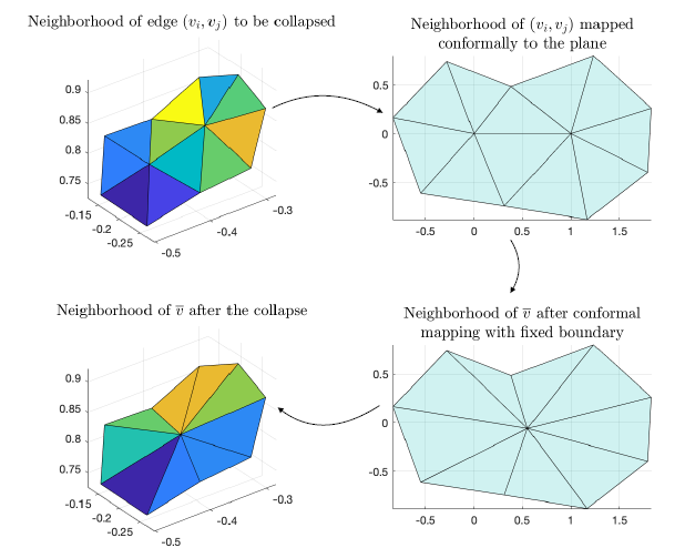
For each edge collapse, we use this procedure to create a bijective mapping between the original mesh, called \(\mathcal{M}^L\), and the mesh after an edge collapse, \(\mathcal{M}^{L-1}\). To construct a mapping from our coarsest mesh to finest mesh, we used spectral conformal parameterization as described in Mullen et al. 2008 [3] and build a successive mapping following the same procedure as Liu et al. 2020 [7]. As mentioned in the previous section, conformal mapping is a parameterization method that preserves angles. For a single edge collapse, \(\mathcal{M}^L\) and \(\mathcal{M}^{L-1}\) are the same except for the neighborhood of the collapsed edge. Therefore, if \((v_i,v_j)\) is the edge to be collapsed, we only need to build a mapping from the neighborhood of \((v_i,v_j)\) in \(\mathcal{M}^L\) to the neighborhood of \(\overline{v}\) in \(\mathcal{M}^{L-1}\). We do this in three steps:
We first map the neighborhood of \((v_i,v_j)\) to the plane via conformal mapping.
A key observation here is that the neighborhood of \(\overline{v}\in\mathcal{M}^{L-1}\) has the same boundary as the neighborhood of \((v_i,v_j)\) before the collapse. We then do a conformal mapping of the neighborhood of \(\overline{v}\in\mathcal{M}^{L-1}\) fixing the boundary so that the resulting 2D region is the same as before.
Now we map points between the 3D neighborhoods using the shared 2D domain.
This process is illustrated in Figure 4.
Figure 4: a triangle mesh before and after the collapse (left column) and their corresponding parameterizations (right column). By mapping the mesh before and after the collapse to the plane, it is possible to create a bijective mapping between the two meshes.
We repeat this process successively for a certain number of collapses to arrive at the desired, coarsest mesh. We refer to the combination of these methods as successive self-parameterization, as described in Liu et al. 2020 [7]. In the implementation of our algorithm, we ran into problems with overlapping faces and badly shaped, skinny triangles. We discuss the mitigation of these problems in the next section.
V. Testing And Improvements
In each part of the project, we always tried to test and potentially improve its results. These helped improve the final output as discussed in Section VI – Results.
V.1. Quality checks for avoiding skinny triangles
To help solve the problem of skinny triangles, we implemented a quality check on the triangles of our mesh post-collapse using the following formula:
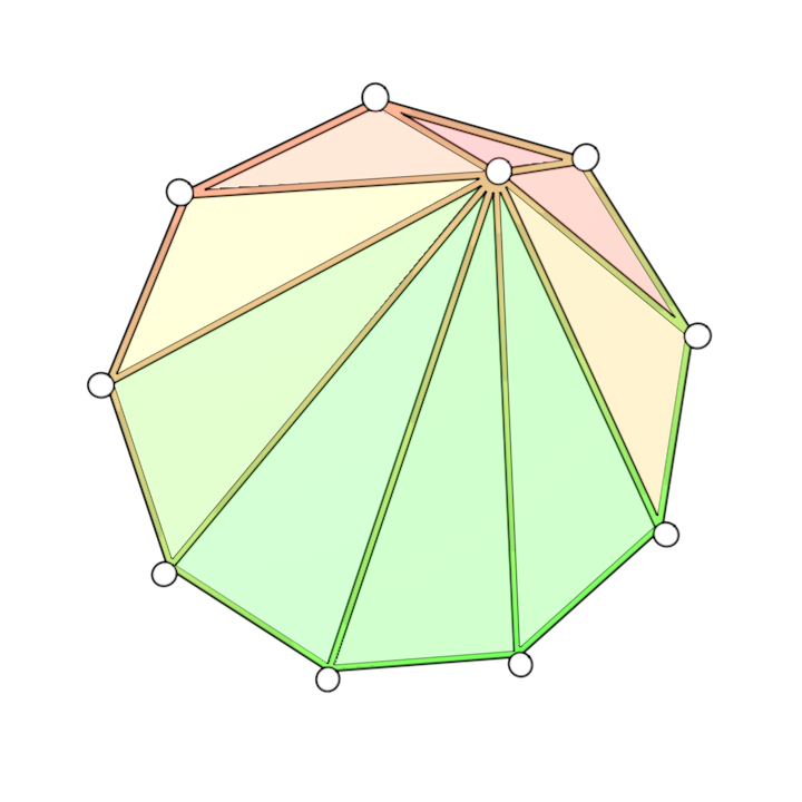
Here \(A\) is the area of a triangle, \(l\) are the lengths of the triangle edges, and \(i,j,k\) represent the indices of the vertices on the triangle. Values of \(Q\) closer to 1 indicate a high quality triangle, while values nearing 0 indicate a degenerate, poor quality triangle. We implemented a test that undoes a collapse if any of the triangles generated have a low value of \(Q_{ijk}\). Figure 5 shows an image with faces of varying quality. Red indicates low quality while green indicates high quality.
Figure 5: visualization of the quality of each triangle in a triangle mesh. A red triangle represents bad quality while a green triangle represents good quality.
V.2. The Delaunay Condition and Edge flips for avoiding skinny triangles
After testing the pipeline on multiple meshes and with different parameters, we realized that there was one issue. While the up-sampled mesh had good geometric quality (due to successive self-parameterization), the triangle quality was not very good. This is because the edge collapses can generally produce some skinny triangles.
To solve this, we implemented a local edge flip after each edge collapse. In that case, we check for edges that don’t satisfy the Delaunay Condition. The Delaunay condition is a good way to improve the triangle angles by penalizing obtuse angles.
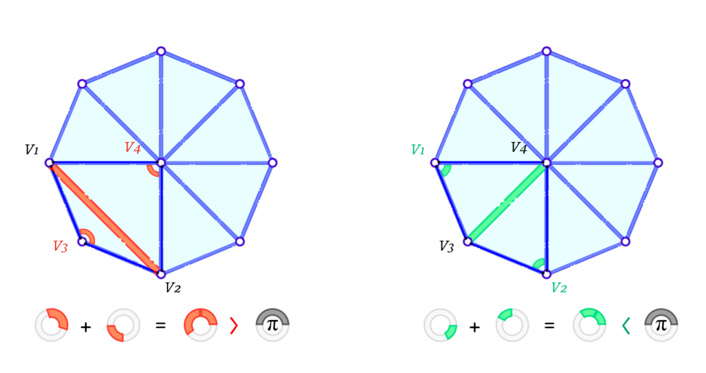
Figure 6: example of a mesh that does not satisfy the Delaunay condition (left) and of a mesh that does satisfy the Delaunay condition (right).
Figure 6 illustrates two cases where the left one violates the Delaunay condition while the one on the right satisfies it. Formally, for a given interior edge \(e_{1-2}\) connecting the vertices \(v_1\) and \(v_2\), and having \(v_3\) and \(v_4\) opposite to it on each of its 2 faces, it satisfies the condition if and only if the sum of the 2 opposite interior angles is less than or equal to \(\pi\). In other words:
As this makes it very unlikely to have obtuse angles, it eliminates some cases of skinny triangles. It is important to note that a skinny triangle can be produced even if all angles are acute, as one of them can be a very small angle. This is another case of skinny triangles but we have other checks mentioned before to help avoid such cases.
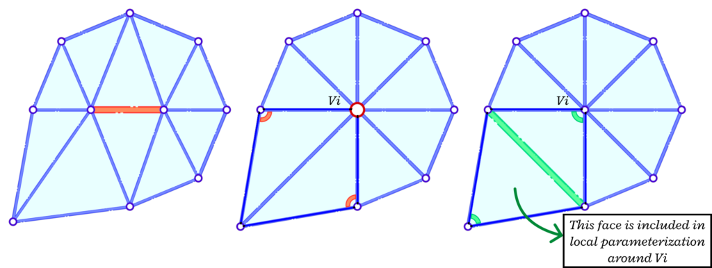
Figure 7: given an initial mesh (left), the edge collapse may generate skinny triangles (center). The edges of the triangles that violate the Delaunay condition are flipped (right).
The edge flips are implemented right before the self-parameterization part. This is to improve triangle quality after each collapse. The candidate edges for a flip are only the ones that are connected to the vertex resulting from the collapse. We also need a copy of the face list before the flip to ensure the neighbourhood is consistent before and after the collapse when we go into the self-parameterization stage. Figure 7 shows an example of a consistent neighbourhood before the collapse, after the edge collapse and after the edge flip (in that order). We need to consider the face that is not any more a neighbor to the vertex to have a consistent mapping.
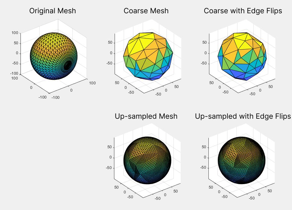
The addition of edge flips improved the triangle quality of the final mesh (after re-sampling for remeshing). Figure 8 shows an example of this on a UV sphere. A quantitative analysis of the improvement is also discussed in the Results section.
Figure 8: visual comparison between the results of mesh simplification without edge flip (center column) and with edge flip (right column).
V.3. Preventing UV faces overlaps
According to Liu et al. 2020 [7], even with consistently oriented faces in the Euclidean and parameterized spaces, it is still possible that two faces overlap each other in the parameterized space. To prevent this artifact, the authors propose to check, in the UV domain, if an interior vertex of the edge to be collapsed has a total angle over \(2 \pi\). If this condition is satisfied, then the edge should not collapse. However, it may also be the case that the condition is satisfied after the collapse. In this case, this edge collapse must be undone and a different edge must be collapsed.
VI. Results
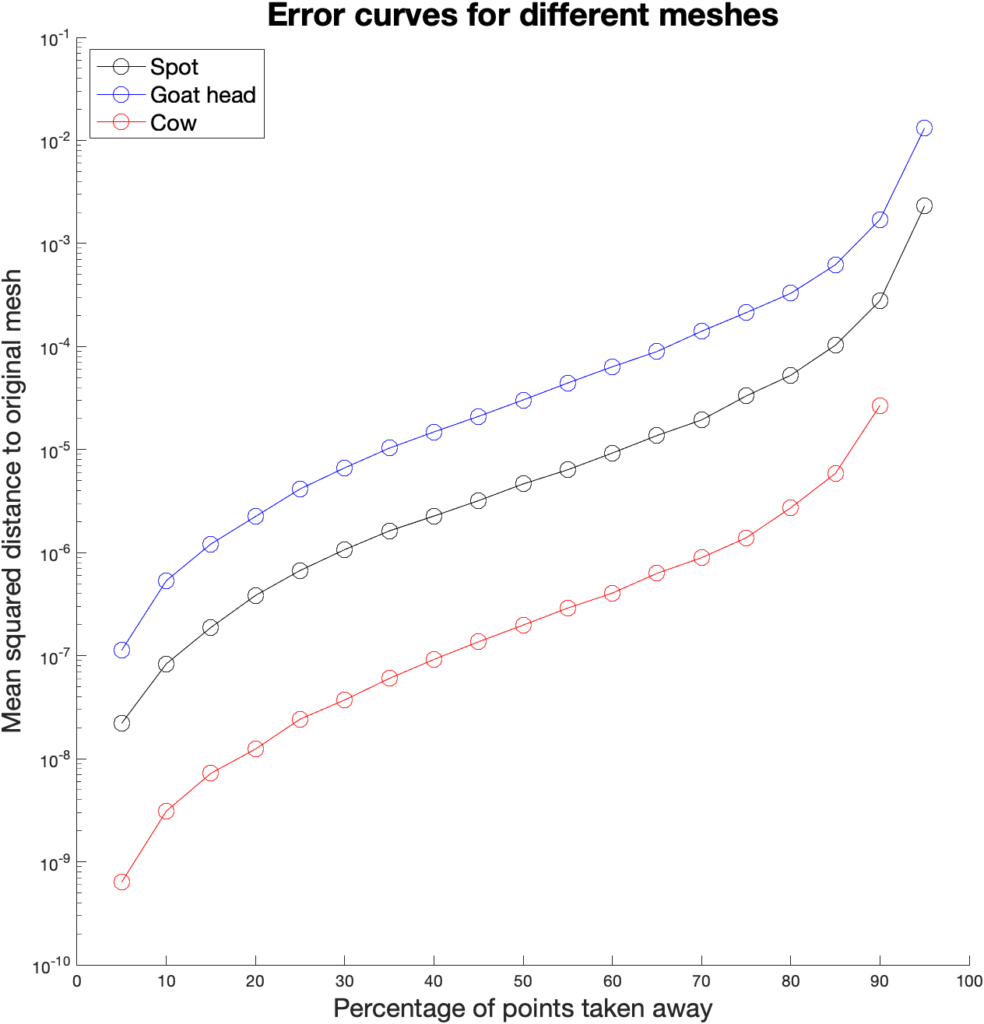
During this project we designed a procedure which can simplify any mesh via edge collapses as we have seen in all the animations. Figure 9 shows how well the coarse mesh approximates the original.
Figure 9: mean square distance between the original mesh and successive meshes in the hierarchy of meshes, built through mesh simplification.
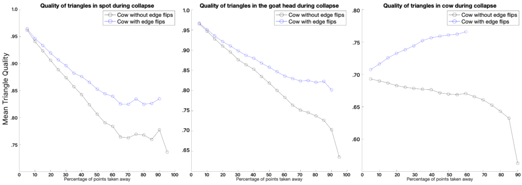
Another thing we measured was the quality of the mesh produced. Depending on the application, different measurements can be done. In our case, we have followed Liu et al. 2020 [7], which uses the quality measure \(Q_{ijk}\) defined in Section V.1. We average \(Q_{ijk}\) over all triangles in a mesh and plot the results across the percentage of vertices removed by edge collapses. Figure 10 shows the results for three different models.
Figure 10: variation of mean average quality along the hierarchy of meshes for three different models.
After the removal of approximately \(65 \%\) of the initial number of vertices, we notice that all meshes begin to level out and there is even marginal improvement for Spot the Cow model. Furthermore, we observe that the implementation of edge flips significantly increases the quality of the meshes produced. Unfortunately, we weren’t able to exploit its full capacity due to a lack of time and a bug in the code.
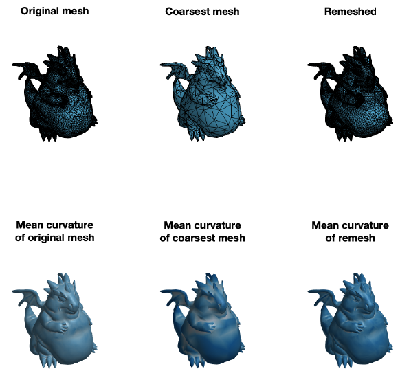
Finally, we have applied the self parameterization to perform remeshing. We have built a bijection \(\mathcal{M}^0\overset{f}{\longrightarrow}\mathcal{M}^L\) where \(\mathcal{M}^0\) is the coarsest mesh and \(\mathcal{M}^L\) is the original mesh. To remesh, we first upsample the topology of the coarse mesh \(M^{0}\), which adds more vertices and faces to the mesh. Subsequently, we use the bijective map to find correspondences between the upsampled mesh and the original mesh. With this correspondence, we build a new mesh with vertices lying inside the original. Figure 11 shows the result of the simplification followed by the remeshing process.
Figure 11: result of applying successive self-parameterization for remeshing. Given an initial fine mesh (left), it is simplified to a target number of faces (center). Then, this coarsest mesh is remeshed to match the original fine mesh (right). In the bottom row we can see the effect that this application has on the mean curvature.
VII. Conclusions and Future Work
In this project we explored hierarchical surface representations combined with successive self-parameterization, using mesh simplification to build a hierarchy of meshes and successive conformal mappings to build correspondences between different levels of the hierarchy. This allows to represent a surface with distinct levels of detail depending on the application. We investigated the application of the successive self-parameterization for remeshing and evaluated various quality metrics on the hierarchy of meshes, which provides meaningful insight into the preservation and loss of geometric data caused by the simplification process.
As main lines of future work, we envision using the successive self-parameterization to solve Poisson equations on curved surfaces, as done by Liu et al. 2021 [8]. While not yet complete, we started the implementation of the intrinsic prolongation operator, which is required for the geometric multigrid method to transfer solutions from coarse to fine meshes. Another step in this project could be creating a texture mapping between the course and fine mesh. Finally, another direction could be remeshing according to the technique using wavelets described in Khodakovsky et al. 2000 [1]. In this paper, wavelets are used to represent the difference between the coarsest and finest levels of a mesh.
While working on the application of Remeshing, that is, using the coarse mesh with upsampling and using the local information stored to reconstruct the geometry, we found that the edge flips after each collapse to be very promising. Based on that, we believe a more robust implementation of this idea can give better results in general. Moreover, we can use other remeshing operations when necessary. For example, tangential relaxation, edge splits and other operations might be useful for getting better-quality triangles. We have to be careful about how and when to apply edge splits, as applying them in each iteration would slow down the collapse convergence.
Another important line of work would be to improve performance and memory consumption in our implementation. While many operations were fully vectorized, there are still areas that can be improved.
We want to thank Professor Paul Kry for the guidance and mentorship (and patience on MATLAB debugging sessions) during these weeks. It is incredible how much can be learned and achieved in a short period of time with an enthusiastic mentor. We also want to thank the volunteers Leticia Mattos Da Silva and Erik Amézquita for all the tips and help they provided. Finally, we would like to thank Professor Justin Solomon for organizing SGI and making it possible to have a fantastic project with students and mentors from all over the world.
VIII. References
[1] Khodakovsky, A., Schröder, P., & Sweldens, W. (2000, July). Progressive geometry compression. In Proceedings of the 27th annual conference on Computer graphics and interactive techniques (pp. 271-278).
[2] Lee, A. W., Sweldens, W., Schröder, P., Cowsar, L., & Dobkin, D. (1998, July). MAPS: Multiresolution adaptive parameterization of surfaces. In Proceedings of the 25th annual conference on Computer graphics and interactive techniques (pp. 95-104).
[3] Mullen, P., Tong, Y., Alliez, P., & Desbrun, M. (2008, July). Spectral conformal parameterization. In Computer Graphics Forum (Vol. 27, No. 5, pp. 1487-1494). Oxford, UK: Blackwell Publishing Ltd.
[4] Lévy, Bruno, et al. “Least squares conformal maps for automatic texture atlas generation.” ACM transactions on graphics (TOG) 21.3 (2002): 362-371.
[5] Hoppe, H., DeRose, T., Duchamp, T., McDonald, J., & Stuetzle, W. (1993, September). Mesh optimization. In Proceedings of the 20th annual conference on Computer graphics and interactive techniques (pp. 19-26)
[6] Garland, M., & Heckbert, P. S. (1997, August). Surface simplification using quadric error metrics. In Proceedings of the 24th annual conference on Computer graphics and interactive techniques (pp. 209-216).
[7] Liu, H., Kim, V., Chaudhuri, S., Aigerman, N. & Jacobson, A. Neural Subdivision. ACM Trans. Graph.. 39 (2020)
[8] Liu, H., Zhang, J., Ben-Chen, M. & Jacobson, A. Surface Multigrid via Intrinsic Prolongation. ACM Trans. Graph.. 40 (2021)
[9] Levoy, M., Pulli, K., Curless, B., Rusinkiewicz, S., Koller, D., Pereira, L., Ginzton, M., Anderson, S., Davis, J., Ginsberg, J. & Others The digital Michelangelo project: 3D scanning of large statues. Proceedings Of The 27th Annual Conference On Computer Graphics And Interactive Techniques. pp. 131-144 (2000)
[10] Hormann, K., Lévy, B. & Sheffer, A. Mesh parameterization: Theory and practice. (2007)
[11] Li, W., Ray, N. & Lévy, B. Automatic and interactive mesh to T-spline conversion. 4th Eurographics Symposium On Geometry Processing-SGP 2006. (2006)
[12] Konaković, M., Crane, K., Deng, B., Bouaziz, S., Piker, D. & Pauly, M. Beyond developable: computational design and fabrication with auxetic materials. ACM Transactions On Graphics (TOG). 35, 1-11 (2016)
[13] Desbrun, M., Meyer, M. & Alliez, P. Intrinsic parameterizations of surface meshes. Computer Graphics Forum. 21, 209-218 (2002)