By SGI Fellows: Anna Cole, Francisco Unai Caja López, Matheus da Silva Araujo, Hossam Mohamed Saeed
I. Introduction
In this project, mentored by Professor Paul Kry, we are exploring properties and applications of multiresolution surface representations: surface meshes with different complexities and details that represent the same underlying surface.
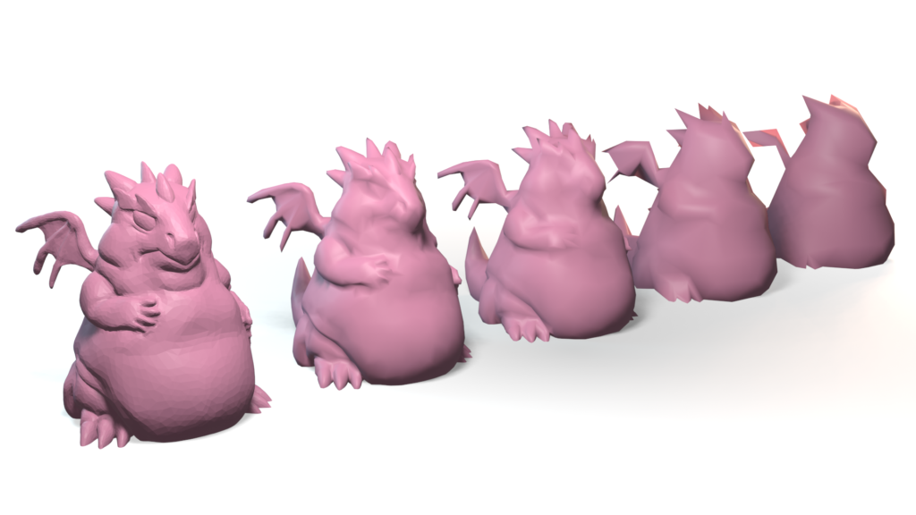
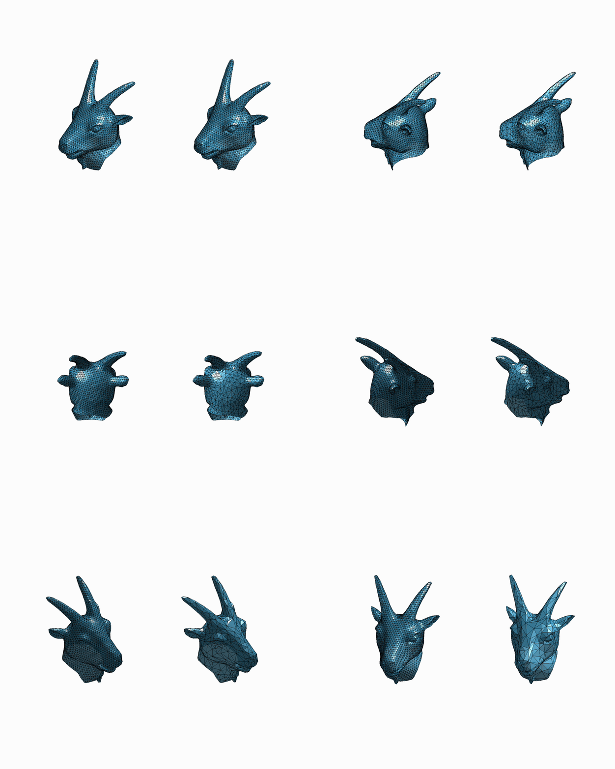
Frequently, the digital representation of intricate and detailed surfaces requires huge triangle meshes. For instance, the digital scan of Michelangelo’s statue of David [9] contains over 1 billion polygon faces and requires 32 GB of memory. The high level of complexity makes it costly to store and render the surface. Furthermore, applying standard geometry processing algorithms on such complex meshes requires huge computational resources. An alternative consists in representing the underlying surface using hierarchy of meshes, also known as multiresolution representations [2]. Each successive level of the hierarchy uses a mesh with lower geometric complexity while representing the same smooth surface. A hierarchy of meshes allows to represent surfaces at different resolutions, which is critical to handle complex geometric models. This form of representation provides efficiency and scalability for rendering and processing of complex surfaces, because the level of detail of the surface can be adjusted based on the hardware available. Figure 1 shows one example of a hierarchy of meshes. In this project we explore the construction of hierarchical representations of surface meshes combined with correspondences between different levels of the hierarchy.
One critical point of this construction is a mapping between meshes at different levels. Liu et al. 2020 [7] proposes a bijective map, named successive self-parameterization, that allows to correspond coarse and fine meshes on the multiresolution hierarchy. To build this mapping, successive self-parameterization requires a (i) mesh simplification algorithm to build the hierarchy of meshes and (ii) a conformal parameterization to map meshes on successive refinement levels to a common space. Our goal for this project is to investigate different applications of this mapping. In the next sections, we detail the algorithms to construct the hierarchy and the successive self-parameterization.
II. Mesh simplification
II.1. Mesh simplification using quadric error
The mesh simplification algorithm studied was introduced in Garland and Heckbert 1997 [6] and is quite straightforward: it consists in collapsing various edges of the mesh sequentially. Specifically, in each iteration, two neighboring vertices \(v_i\) and \(v_j\) will be chosen and replaced by a single vertex \(\overline{v}\). The new vertex \(\overline{v}\) will inherit all neighbors of \(v_i\) and \(v_j\). In Animation 1 it is possible to see the possible result of two edge collapses in a triangle mesh.
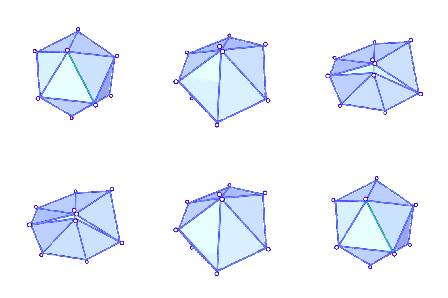
Suppose we have decided to collapse edge \((v_i,v_j)\). Then, \(\overline{v}\) is found as the solution of a minimization problem. For each vertex \(v_i\) we define a matrix \(Q_i\) so that \(v^TQ_iv\), with \(v=[v_x, v_y, v_z, 1]\), gives a measure of how far \(v\) is from \(v_i\). We choose \(\overline{v}\) minimizing \(v^T(Q_i+Q_j)v\). As for the choice of the \(Q\) matrices, we consider:
- To each vertex \(v_i\) we associate the set of planes corresponding to faces that contain \(v_i\) and denote it \(\mathcal{P}(v_i)\).
- For each face of the mesh we consider \(p=[a,b,c,d]^T\) such that \(v^Tp=0\) is the equation of the plane and \(a^2+b^2+c^2=1\). This allows us to compute the distance from a point \(v=[v_x,v_y,v_z,1]\) to the plane as \(\vert v^Tp \vert\).
Then, the sum of the squared distances from \(v\) to each plane in \(\mathcal{P}(v_i)\) would be
\(\displaystyle \sum_{p\in\mathcal{P}(v_{i})}(v^{T}p)^{2}= \sum_{p\in\mathcal{P}(v_{i})}v^{T}pp^{T}v = v^{T}\Bigg(\underbrace{\sum_{p\in\mathcal{P}(v_{i})}pp^{T}}_{{\text{choice of} }Q_{i}}\Bigg)v\)
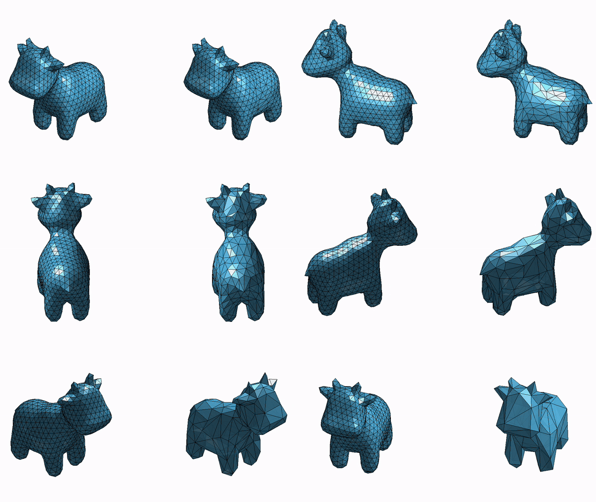
Finally, we decide which edge to collapse by choosing \((v_i,v_j)\) minimizing the error \(\overline{v}^T(Q_i+Q_j)\overline{v}\). For the following iterations, \(\overline{v}\) is assigned the matrix \(Q_i+Q_j\). Animations 2 and 3 illustrates the process of mesh simplification using quadric error.
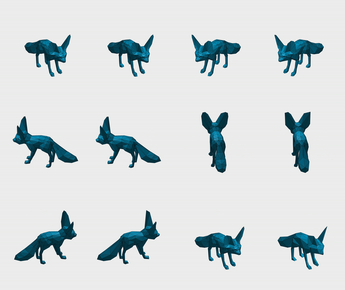
The algorithm can also run on meshes with boundaries. In Animation 4 we chose not to collapse boundary edges, which allows the boundaries to be preserved.
II.2. Manifoldness and edge collapse validation
There are a variety of issues that can occur if we collapse each edge only based on the error quadrics \(Q_i+Q_j\). This is because the error quadric is only concerned with the geometry of the meshes but not the topology. So we needed to implement some connectivity checks to make sure the edge collapse wouldn’t result in a non-manifold case or change the topology of the mesh.
This can be visualized in Animation 5, where collapsing an interior edge consisting of two boundary vertices can create a non-manifold edge (or vertex). Another problematic case is collapsing an edge with its two vertices sharing more than two neighboring vertices, which would break manifoldness. We followed the criteria described in Liu et al. 2020 [7] and Hoppe el al. 1993 [5] to guarantee an manifold input mesh stays manifold after each collapse. Also, we added the condition where we compute the Euler characteristic \(\chi(M)\) before and after the collapse and if there is a change, we revert back and choose a different edge. In case all remaining edges are not valid for the collapse operation, we simply stop the collapsing process and move on to the next step.
III. Mesh parameterization
Mesh parameterization deals with the problem of mapping a surface to the plane. In our case, the surface is represented by a triangle mesh. This means that for every vertex of the triangle mesh we find corresponding coordinates on the 2D plane. More precisely, given a triangle mesh \(\mathcal{M}\), with a set of vertices \(\mathcal{V}\) and a set of triangles \(\mathcal{T}\), the mesh parameterization problem is concerned with finding a map \(f: \mathcal{V} \rightarrow \Omega \subset \mathbb{R}^{2}\). The effect of this mapping can be seen in Animation 6, where one 3D mesh is flattened to the 2D plane.
This mapping enables all sorts of interesting applications. The most famous one is texture mapping: how to specify texture coordinates for each vertex of a triangle mesh such that you can map a region of an image to the mesh? Other applications include conversion of triangle meshes into parametric surfaces [11] e.g., T-Splines or NURBS and computational fabrication [12]. In this section we won’t give all the details about this field, but rather will focus on the aspects relevant to build mappings between meshes of different refinement levels on the hierarchical surface representation. We refer the interested reader to Hormann et al. 2007 [10] for an extensive treatment.
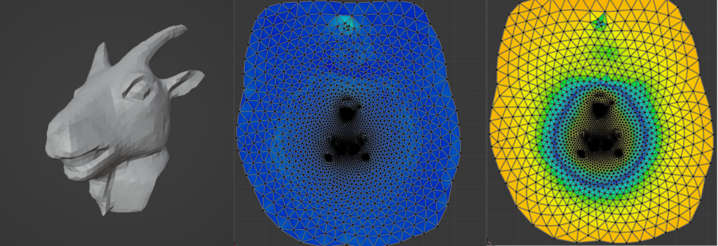
There are many different possibilities to define the mapping from the surface to the plane. However, this mapping usually introduces undesirable distortions. Depending on the construction used, the map may preserve areas, but not angles or orientations; conversely, it may preserve angles but not areas and lengths. This can be seen in Figure 2, where we can visualize angles and area distortions in the parameterized mesh.
To create maps between meshes of different levels, Liu et al. 2020 [7] uses conformal mappings, which are maps that preserve angles. Conformal mappings are efficient to compute and provide theoretical guarantees, making it a common choice for many geometry processing tasks.
A conformal map is characterized by the Cauchy-Riemann equations:
\(\displaystyle \begin{align*} \frac{\partial v(x,y)}{\partial x} &= -\frac{\partial u(x,y)}{\partial y} \\ \frac{\partial v(x,y)}{\partial y} &= \frac{\partial u(x,y)}{\partial x} \end{align*}\)
or, more compactly,
\(\nabla u = \nabla v^{\bot}\)
Conformal mappings also have a strong connection with complex analysis, which leads to an alternative but equivalent formulation of the problem.
For arbitrary triangle meshes it is impossible to find an exact conformal mapping; only developable meshes (i.e., meshes with zero Gaussian curvature at every point) can be conformally parameterized. In most cases, this restriction is too severe. To work around this, it is possible to build a conformal mapping satisfying the previous equations as close as possible. In other words, we can associate it with an energy function to find the mapping that better approximates a conformal mapping using a least squares formulation:
\(E_{LSCM} = \int_{\mathbf{S}} \lVert \nabla u – \nabla v^{\bot} \rVert^2 dA\)
where \(S\) is the smooth surface represented by a triangle mesh \(\mathcal{M}\).
On a triangle mesh, the functions \(u(x, y), v(x,y)\) can be written with respect to the local orthonormal coordinate system of the triangle. Since the triangle mesh is a piecewise linear surface, the gradient of a function defined over the mesh is constant with respect to each triangle. This makes it possible to find the mapping that better approximates the Cauchy-Riemann equations for each triangle of the mesh. Hence, in this discrete setting, the previous equation can be rewritten as follows
\(\displaystyle \begin{align*} E_{LSCM} &= \sum_{t \in \mathcal{T}} A_{t} \left \lVert M_{t} \cdot \mathbf{v}_{t} – \begin{bmatrix}0 & -1 \\ 1 & 0 \end{bmatrix} M_{t} \cdot \mathbf{u}_{t} \right \rVert ^{2} \\ M_{t} &= \frac{1}{2 \cdot A_{t}} \cdot \begin{bmatrix} y_{j} – y_{k} & y_{k} – y_{i} & y_{i} – y_{j}\\ x_{k} – x_{j} & x_{i} – x_{k} & x_{j} – x_{i} \end{bmatrix} \end{align*}\)
where \(A_{t}\) denotes the area of each triangle with vertices represented by \((i, j, k)\). The solution of the discrete conformal energy described above are the coordinates \((u, v)\) in the 2D plane for each vertex of each triangle \(t\) in the set of triangles \(\mathcal{T}\) of the mesh \(\mathcal{M}\). More details can be found in Lévy et al. 2002 [4] and Desbrun et al. 2002 [13].
However, the trivial solution for this equation would be to set all coordinates \((u, v)\) to the same point and the energy would be minimized, which is not what we want. Therefore, to prevent this case, it is necessary to fix or pin two arbitrary vertices to arbitrary positions in the plane. This restriction generates a least squares problem with a unique solution. The choice of the vertices to be fixed is arbitrary but can have impact on the quality and numerical stability of the parameterization. For instance, there can be arbitrary area distortions depending on the vertices that are fixed. To prevent the problem of the trivial solution while preserving numerical stability, an alternative strategy is proposed by Mullen et al. 2008 [3] in which the system is reformulated to an equivalent eigendecomposition problem which avoid the need to pin any vertex.
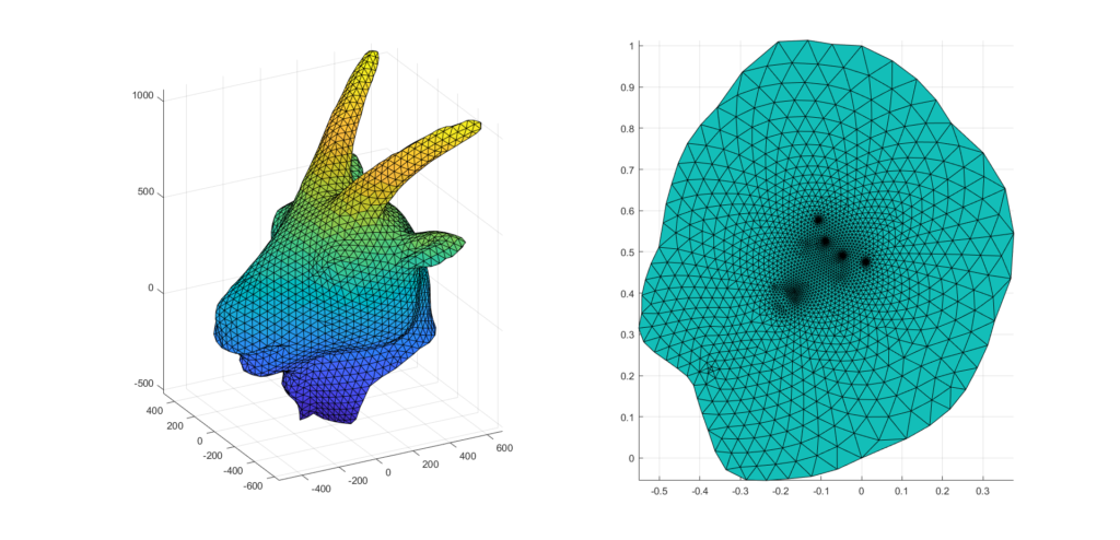
Figure 3 illustrates the least squares conformal mapping obtained for a triangle mesh with boundaries. Notice that the map obtained doesn’t necessarily preserve areas and lengths. Furthermore, as can be seen in the right plot of the figure, lots of details are grouped around tiny regions in the interior of the parameterized mesh.
This algorithm is a central piece to create a bijective map between meshes on different levels of the hierarchy.
IV. Successive self-parameterization
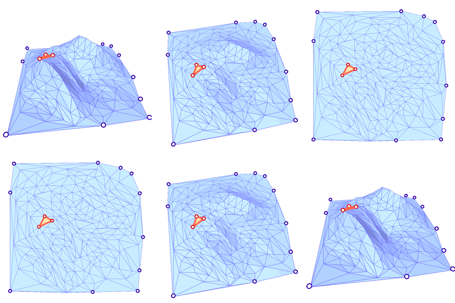
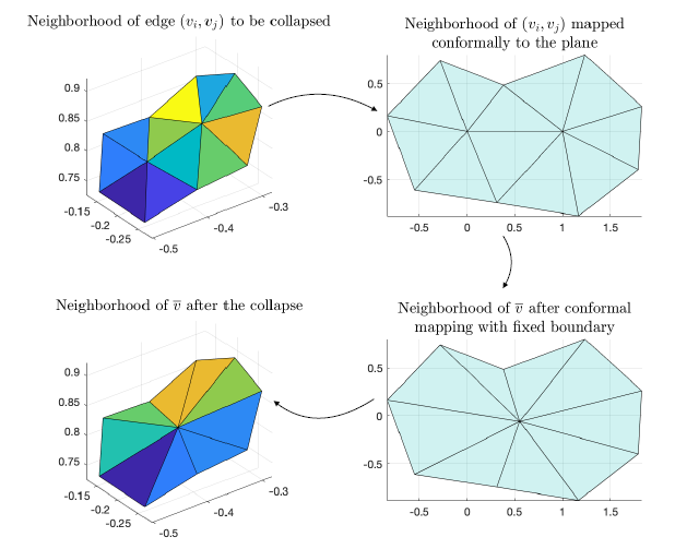
For each edge collapse, we use this procedure to create a bijective mapping between the original mesh, called \(\mathcal{M}^L\), and the mesh after an edge collapse, \(\mathcal{M}^{L-1}\). To construct a mapping from our coarsest mesh to finest mesh, we used spectral conformal parameterization as described in Mullen et al. 2008 [3] and build a successive mapping following the same procedure as Liu et al. 2020 [7]. As mentioned in the previous section, conformal mapping is a parameterization method that preserves angles. For a single edge collapse, \(\mathcal{M}^L\) and \(\mathcal{M}^{L-1}\) are the same except for the neighborhood of the collapsed edge. Therefore, if \((v_i,v_j)\) is the edge to be collapsed, we only need to build a mapping from the neighborhood of \((v_i,v_j)\) in \(\mathcal{M}^L\) to the neighborhood of \(\overline{v}\) in \(\mathcal{M}^{L-1}\). We do this in three steps:
- We first map the neighborhood of \((v_i,v_j)\) to the plane via conformal mapping.
- A key observation here is that the neighborhood of \(\overline{v}\in\mathcal{M}^{L-1}\) has the same boundary as the neighborhood of \((v_i,v_j)\) before the collapse. We then do a conformal mapping of the neighborhood of \(\overline{v}\in\mathcal{M}^{L-1}\) fixing the boundary so that the resulting 2D region is the same as before.
- Now we map points between the 3D neighborhoods using the shared 2D domain.
This process is illustrated in Figure 4.
We repeat this process successively for a certain number of collapses to arrive at the desired, coarsest mesh. We refer to the combination of these methods as successive self-parameterization, as described in Liu et al. 2020 [7]. In the implementation of our algorithm, we ran into problems with overlapping faces and badly shaped, skinny triangles. We discuss the mitigation of these problems in the next section.
V. Testing And Improvements
In each part of the project, we always tried to test and potentially improve its results. These helped improve the final output as discussed in Section VI – Results.
V.1. Quality checks for avoiding skinny triangles
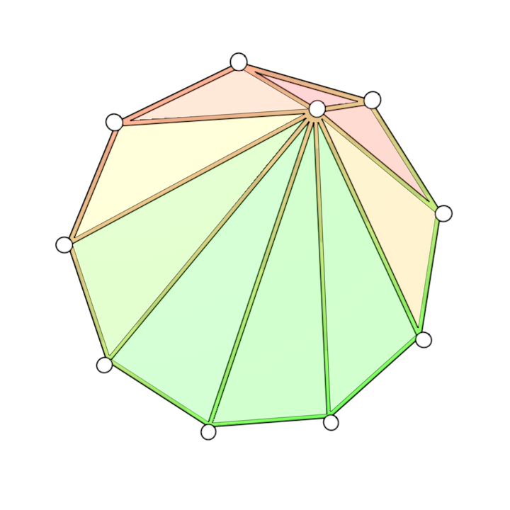
To help solve the problem of skinny triangles, we implemented a quality check on the triangles of our mesh post-collapse using the following formula:
\(Q_{ijk}=\frac{4\sqrt{3}A_{ijk}}{l_{ij}^2+l_{jk}^2+l_{ki}^2}\)
Here \(A\) is the area of a triangle, \(l\) are the lengths of the triangle edges, and \(i,j,k\) represent the indices of the vertices on the triangle. Values of \(Q\) closer to 1 indicate a high quality triangle, while values nearing 0 indicate a degenerate, poor quality triangle. We implemented a test that undoes a collapse if any of the triangles generated have a low value of \(Q_{ijk}\). Figure 5 shows an image with faces of varying quality. Red indicates low quality while green indicates high quality.
V.2. The Delaunay Condition and Edge flips for avoiding skinny triangles
After testing the pipeline on multiple meshes and with different parameters, we realized that there was one issue. While the up-sampled mesh had good geometric quality (due to successive self-parameterization), the triangle quality was not very good. This is because the edge collapses can generally produce some skinny triangles.
To solve this, we implemented a local edge flip after each edge collapse. In that case, we check for edges that don’t satisfy the Delaunay Condition. The Delaunay condition is a good way to improve the triangle angles by penalizing obtuse angles.
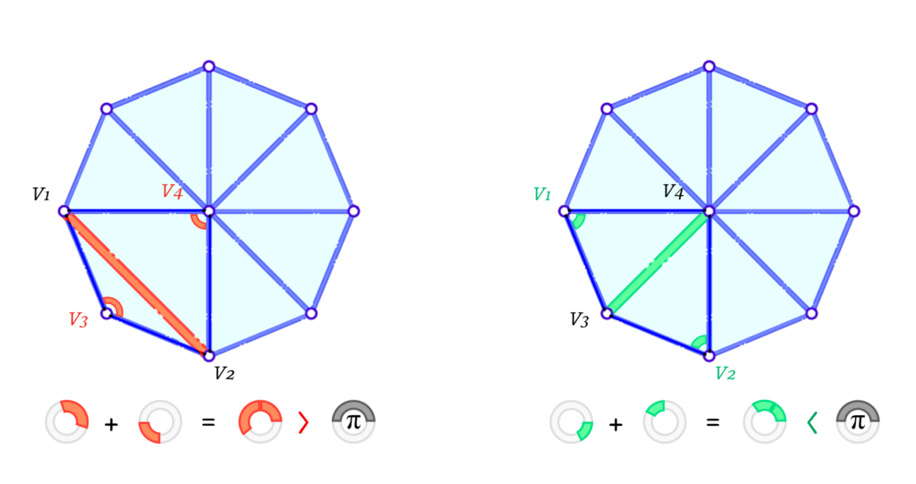
Figure 6 illustrates two cases where the left one violates the Delaunay condition while the one on the right satisfies it. Formally, for a given interior edge \(e_{1-2}\) connecting the vertices \(v_1\) and \(v_2\), and having \(v_3\) and \(v_4\) opposite to it on each of its 2 faces, it satisfies the condition if and only if the sum of the 2 opposite interior angles is less than or equal to \(\pi\). In other words:
\(\angle v_1 v_4 v_2 + \angle v_2 v_3 v_4 \leq \pi\)
As this makes it very unlikely to have obtuse angles, it eliminates some cases of skinny triangles. It is important to note that a skinny triangle can be produced even if all angles are acute, as one of them can be a very small angle. This is another case of skinny triangles but we have other checks mentioned before to help avoid such cases.
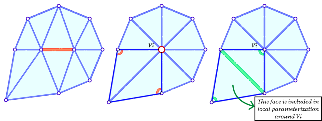
The edge flips are implemented right before the self-parameterization part. This is to improve triangle quality after each collapse. The candidate edges for a flip are only the ones that are connected to the vertex resulting from the collapse. We also need a copy of the face list before the flip to ensure the neighbourhood is consistent before and after the collapse when we go into the self-parameterization stage. Figure 7 shows an example of a consistent neighbourhood before the collapse, after the edge collapse and after the edge flip (in that order). We need to consider the face that is not any more a neighbor to the vertex to have a consistent mapping.
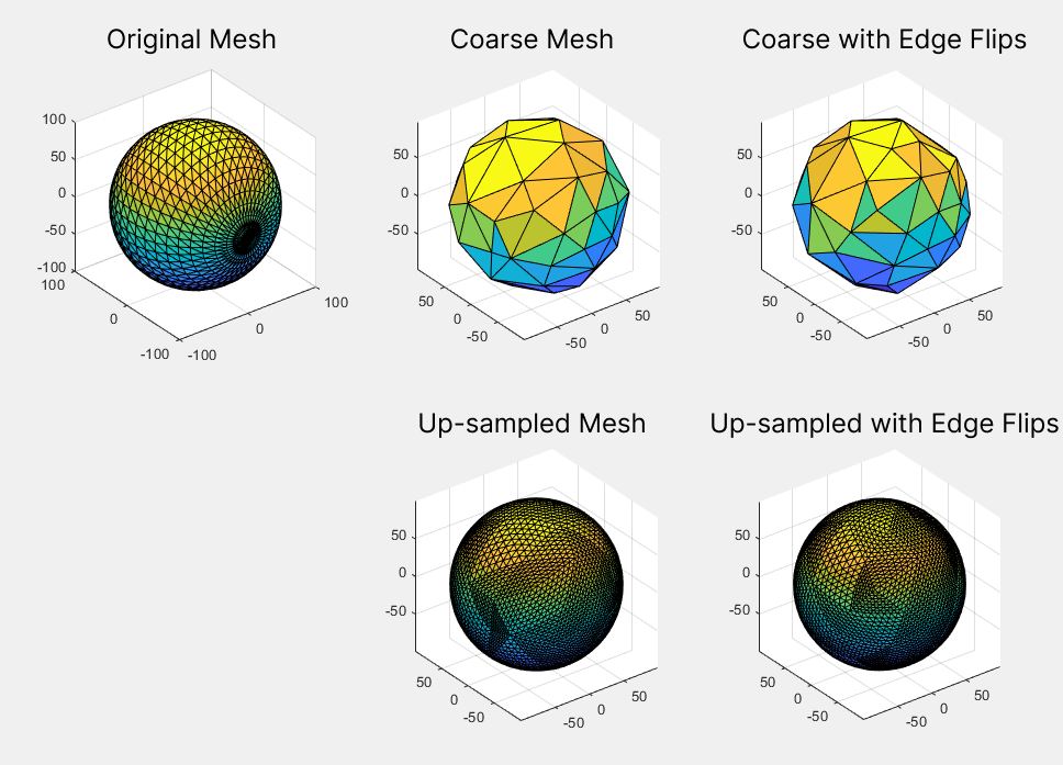
The addition of edge flips improved the triangle quality of the final mesh (after re-sampling for remeshing). Figure 8 shows an example of this on a UV sphere. A quantitative analysis of the improvement is also discussed in the Results section.
V.3. Preventing UV faces overlaps
According to Liu et al. 2020 [7], even with consistently oriented faces in the Euclidean and parameterized spaces, it is still possible that two faces overlap each other in the parameterized space. To prevent this artifact, the authors propose to check, in the UV domain, if an interior vertex of the edge to be collapsed has a total angle over \(2 \pi\). If this condition is satisfied, then the edge should not collapse. However, it may also be the case that the condition is satisfied after the collapse. In this case, this edge collapse must be undone and a different edge must be collapsed.
VI. Results
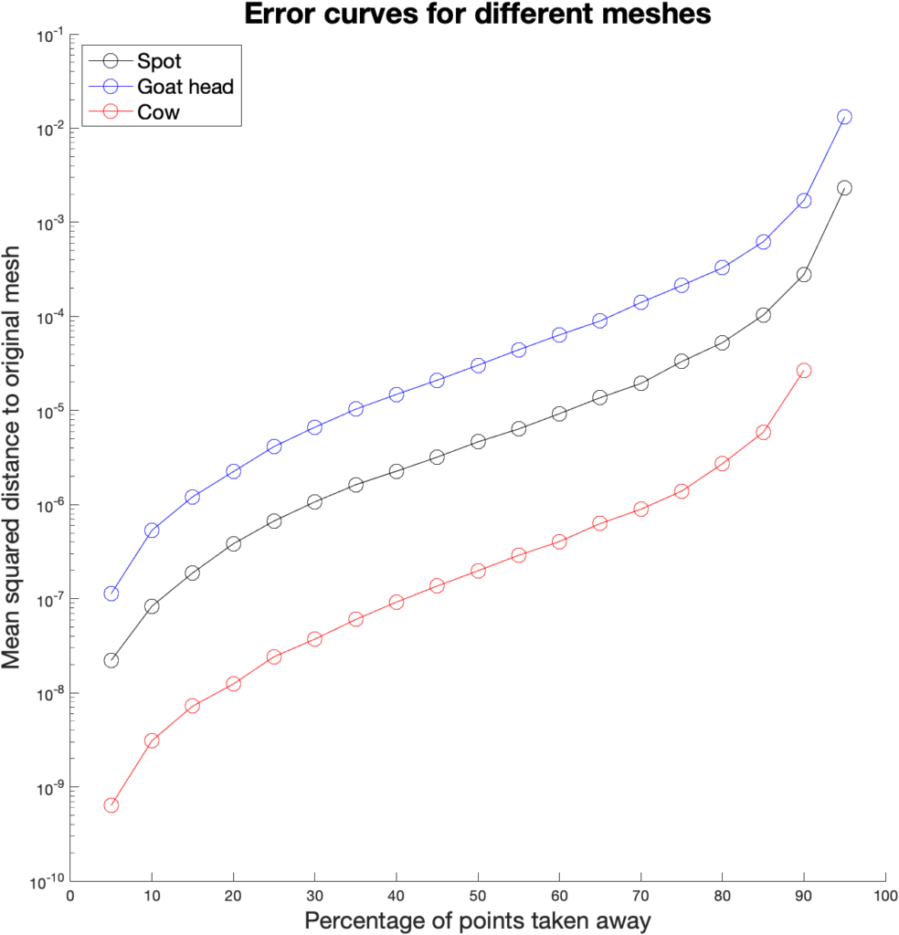
During this project we designed a procedure which can simplify any mesh via edge collapses as we have seen in all the animations. Figure 9 shows how well the coarse mesh approximates the original.
Another thing we measured was the quality of the mesh produced. Depending on the application, different measurements can be done. In our case, we have followed Liu et al. 2020 [7], which uses the quality measure \(Q_{ijk}\) defined in Section V.1. We average \(Q_{ijk}\) over all triangles in a mesh and plot the results across the percentage of vertices removed by edge collapses. Figure 10 shows the results for three different models.
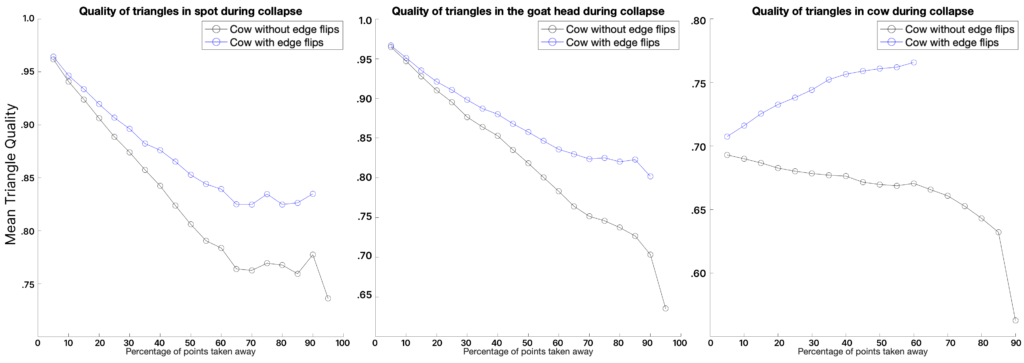
After the removal of approximately \(65 \%\) of the initial number of vertices, we notice that all meshes begin to level out and there is even marginal improvement for Spot the Cow model. Furthermore, we observe that the implementation of edge flips significantly increases the quality of the meshes produced. Unfortunately, we weren’t able to exploit its full capacity due to a lack of time and a bug in the code.
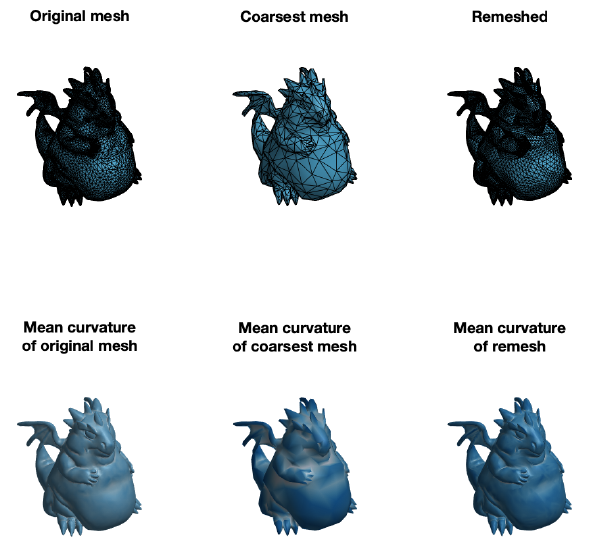
Finally, we have applied the self parameterization to perform remeshing. We have built a bijection \(\mathcal{M}^0\overset{f}{\longrightarrow}\mathcal{M}^L\) where \(\mathcal{M}^0\) is the coarsest mesh and \(\mathcal{M}^L\) is the original mesh. To remesh, we first upsample the topology of the coarse mesh \(M^{0}\), which adds more vertices and faces to the mesh. Subsequently, we use the bijective map to find correspondences between the upsampled mesh and the original mesh. With this correspondence, we build a new mesh with vertices lying inside the original. Figure 11 shows the result of the simplification followed by the remeshing process.
VII. Conclusions and Future Work
In this project we explored hierarchical surface representations combined with successive self-parameterization, using mesh simplification to build a hierarchy of meshes and successive conformal mappings to build correspondences between different levels of the hierarchy. This allows to represent a surface with distinct levels of detail depending on the application. We investigated the application of the successive self-parameterization for remeshing and evaluated various quality metrics on the hierarchy of meshes, which provides meaningful insight into the preservation and loss of geometric data caused by the simplification process.
As main lines of future work, we envision using the successive self-parameterization to solve Poisson equations on curved surfaces, as done by Liu et al. 2021 [8]. While not yet complete, we started the implementation of the intrinsic prolongation operator, which is required for the geometric multigrid method to transfer solutions from coarse to fine meshes. Another step in this project could be creating a texture mapping between the course and fine mesh. Finally, another direction could be remeshing according to the technique using wavelets described in Khodakovsky et al. 2000 [1]. In this paper, wavelets are used to represent the difference between the coarsest and finest levels of a mesh.
While working on the application of Remeshing, that is, using the coarse mesh with upsampling and using the local information stored to reconstruct the geometry, we found that the edge flips after each collapse to be very promising. Based on that, we believe a more robust implementation of this idea can give better results in general. Moreover, we can use other remeshing operations when necessary. For example, tangential relaxation, edge splits and other operations might be useful for getting better-quality triangles. We have to be careful about how and when to apply edge splits, as applying them in each iteration would slow down the collapse convergence.
Another important line of work would be to improve performance and memory consumption in our implementation. While many operations were fully vectorized, there are still areas that can be improved.
We want to thank Professor Paul Kry for the guidance and mentorship (and patience on MATLAB debugging sessions) during these weeks. It is incredible how much can be learned and achieved in a short period of time with an enthusiastic mentor. We also want to thank the volunteers Leticia Mattos Da Silva and Erik Amézquita for all the tips and help they provided. Finally, we would like to thank Professor Justin Solomon for organizing SGI and making it possible to have a fantastic project with students and mentors from all over the world.
VIII. References
[1] Khodakovsky, A., Schröder, P., & Sweldens, W. (2000, July). Progressive geometry compression. In Proceedings of the 27th annual conference on Computer graphics and interactive techniques (pp. 271-278).
[2] Lee, A. W., Sweldens, W., Schröder, P., Cowsar, L., & Dobkin, D. (1998, July). MAPS: Multiresolution adaptive parameterization of surfaces. In Proceedings of the 25th annual conference on Computer graphics and interactive techniques (pp. 95-104).
[3] Mullen, P., Tong, Y., Alliez, P., & Desbrun, M. (2008, July). Spectral conformal parameterization. In Computer Graphics Forum (Vol. 27, No. 5, pp. 1487-1494). Oxford, UK: Blackwell Publishing Ltd.
[4] Lévy, Bruno, et al. “Least squares conformal maps for automatic texture atlas generation.” ACM transactions on graphics (TOG) 21.3 (2002): 362-371.
[5] Hoppe, H., DeRose, T., Duchamp, T., McDonald, J., & Stuetzle, W. (1993, September). Mesh optimization. In Proceedings of the 20th annual conference on Computer graphics and interactive techniques (pp. 19-26)
[6] Garland, M., & Heckbert, P. S. (1997, August). Surface simplification using quadric error metrics. In Proceedings of the 24th annual conference on Computer graphics and interactive techniques (pp. 209-216).
[7] Liu, H., Kim, V., Chaudhuri, S., Aigerman, N. & Jacobson, A. Neural Subdivision. ACM Trans. Graph.. 39 (2020)
[8] Liu, H., Zhang, J., Ben-Chen, M. & Jacobson, A. Surface Multigrid via Intrinsic Prolongation. ACM Trans. Graph.. 40 (2021)
[9] Levoy, M., Pulli, K., Curless, B., Rusinkiewicz, S., Koller, D., Pereira, L., Ginzton, M., Anderson, S., Davis, J., Ginsberg, J. & Others The digital Michelangelo project: 3D scanning of large statues. Proceedings Of The 27th Annual Conference On Computer Graphics And Interactive Techniques. pp. 131-144 (2000)
[10] Hormann, K., Lévy, B. & Sheffer, A. Mesh parameterization: Theory and practice. (2007)
[11] Li, W., Ray, N. & Lévy, B. Automatic and interactive mesh to T-spline conversion. 4th Eurographics Symposium On Geometry Processing-SGP 2006. (2006)
[12] Konaković, M., Crane, K., Deng, B., Bouaziz, S., Piker, D. & Pauly, M. Beyond developable: computational design and fabrication with auxetic materials. ACM Transactions On Graphics (TOG). 35, 1-11 (2016)
[13] Desbrun, M., Meyer, M. & Alliez, P. Intrinsic parameterizations of surface meshes. Computer Graphics Forum. 21, 209-218 (2002)