Visualizing and Evaluating Skin Weight Transfer
My goal for this project was to implement visualization methods that help artists gauge the accuracy of skin weight transfer methods, which takes the skin weights from an already rigged mesh, and assigns the correct weights to the target mesh. I compared two different weight transfer methods. First, Maya’s built-in copySkinWeights: which takes a vertex on the unrigged mesh, finds the closest point on the source mesh, and interpolates the weights at that point to determine the weights at the vertex. Next, a method developed by EpicGames, which copies the weights from the source mesh that have a high-confidence correspondence. For the remaining vertices, it computes the weights by interpolating from the transferred high-confidence weights.
To begin, I downloaded a character with an animation from Mixamo and imported it into Maya. In my first pass comparison, I unbound the shirt from the character, and then rebound it using Maya’s copySkinWeights and EpicGames’ Weight Inpaint method. Below is a playblast of each character. Notice that with the copySkinWeights there is a jagged concave area in the upper back region, while with the Weight Inpaint method, that area is smooth.
Now, I wanted to develop a method to visually compare the two algorithms. I created a heatmap using the error formula.
Expanding on the previous idea, I wanted to develop a dynamic heat map that shows the areas with the highest deformation error over the entire animation. I created a node that took the display/method mesh and reference mesh as inputs, and then took the 3D vertex position of each of the meshes. To calculate the deformation error, I calculated the Euclidean distance between the 3D vertex positions of the method I was evaluating and the 3D vertex position of the original mesh. This is calculated with:
where i represents the ith vertex of the matrix, is the 3D position of vertex i on the method mesh at frame t, is the 3D position of vertex i on the original method at frame t.
To construct the heat map, we normalize and clamp with:
where c is the maximum deformation distance.
We then mapped the errors to colors and wrote all vertex colors to the output mesh with setVertexColors(). We then have our finished output mesh with our desired heatmap. As the animation changes, the input meshes will change, causing the heatmap to update with each frame. This was packaged into a UI for easier use.
Here is the heat map applied to a shirt that was rigged using Maya’s copySkinWeights:
Here is the heat map applied to a shirt that was rigged using EpicGames Inpaint method:
Reference: EpicGames Inpaint Method
TextDeformer: How can words shape the (virtual) world
Researched by: José Pablo Soto Sánchez
Introduction
Imagine handing a sculptor a block of clay and, instead of tools, just a sentence: “make this a giraffe.” No reference photos, no measurements, just words, and the expectation that the clay reshapes itself to match. That’s roughly what TextDeformer (Gao et al., SIGGRAPH 2023) does to a 3D mesh: given a source shape and a target text prompt, it deforms the geometry until a frozen vision-language model agrees that the render looks like the prompt.
What makes this interesting isn’t just the result it’s used purely as a differentiable critic. The actual “learning” happens directly on the geometry: a set of per-triangle Jacobian matrices gets optimized by gradient descent, the same way you’d optimize the weights of a network, except here the “weights” are literally how each triangle is allowed to stretch and rotate.
This post walks through reproducing the official TextDeformer codebase end-to-end on consumer hardware, the math that makes text-to-geometry gradients possible at all, and the specific things that broke along the way and how they got fixed.
Background
A few terms are worth pinning down before the method section, since the pipeline sits at the intersection of graphics and vision-language modeling:
| Term | Plain-language definition |
|---|---|
| CLIP | A frozen, pretrained model that embeds images and text into the same vector space, so cosine similarity between an image embedding and a text embedding measures “how well does this image match this caption.” |
| Differentiable rendering | Turning a 3D mesh + camera into a 2D image using operations (rasterization, shading) that support backpropagation, so pixel-level loss can flow gradients back to vertex positions. |
| Jacobian (per-triangle) | A 3×3 matrix describing how a single triangle is locally stretched/rotated relative to its original shape. TextDeformer optimizes one of these per face, directly. |
| Poisson mesh reconstruction | Given a target Jacobian per triangle, solving a linear system to recover the vertex positions whose actual local deformation best matches those targets, in a least-squares sense. |
| Cotangent Laplacian | A sparse matrix built from mesh geometry that encodes how each vertex relates to its neighbors; it’s the operator at the center of the Poisson solve. |
| ViT patch | A Vision Transformer splits an image into fixed-size square tiles (“patches”) and treats each one like a token — patch size determines how fine-grained the model’s spatial resolution is. |
Method
CLIP-guided losses
The core signal is cosine similarity between a rendered image’s CLIP embedding and the target text’s CLIP embedding:
But optimizing this alone tends to drift toward whatever image maximizes similarity to the prompt, not necessarily a smooth deformation of the source shape. TextDeformer adds a delta-CLIP term that instead matches the change in image embedding against the *change* in text embedding, relative to a fixed base render/prompt (e.g. “a cow”):
This directional formulation (used in prior CLIP-guided editing work) keeps the deformation anchored to the source identity instead of collapsing onto an unrelated “giraffe-like” blob.
Per-triangle Jacobians and the Poisson solve
This is the part that replaces a neural decoder entirely. Given the mesh’s gradient operator (one 3×3 block per face) and a diagonal mass matrix of face areas, the cotangent Laplacian is built as:
has a one-dimensional null space (constant functions), so the implementation drops the first row/column to pin a single vertex before it’s usable for Cholesky factorization. To go from optimized per-face Jacobians back to vertex positions , the code solves the normal equations of a least-squares problem — find the whose actual gradient is as close as possible to the target Jacobians , weighted by face area:
That linear system is factorized once per mesh with a sparse Cholesky solver (`cholespy`, GPU-resident) and re-solved every optimization step as changes — cheap after the one-time factorization. A Jacobian regularization term, , keeps triangles from stretching into degenerate shapes.
Rendering and camera augmentation
Each step, a batch of random cameras (elevation drawn from a Beta distribution, azimuth uniform over 360°, random distance/FOV/lighting/background) renders the current mesh via nvdiffrast‘s differentiable rasterizer. Randomizing viewpoint and lighting every step is what prevents the optimizer from exploiting a single “good” camera angle instead of actually deforming the geometry.
Patch-level consistency loss
A second, separate CLIP ViT is used only for its intermediate patch features (via forward hooks on each transformer block). For pairs of cameras within the same batch that are close in elevation/azimuth, the patches that project to the same 3D vertex are compared — encouraging the same surface point to look consistent from nearby viewpoints, which curbs the multi-view incoherence (“Janus-face”-style artifacts) common to CLIP-guided 3D optimization.
Implementation
Getting the reference implementation running at all.
The repo pins specific commits for nvdiffrast and installs igl unpinned via conda-forge. The unpinned igl immediately caused a break: igl.random_points_on_mesh in MeshProcessor.py expected a 2-tuple return (bary, face_idx), but the installed libigl build now returns a 3-tuple (B, FI, P). Fixed by unpacking a third, unused value — a reminder that “no version pin” in a 2023 paper repo means the API surface has already drifted.
Fighting the GPU context, not the geometry.
The next failure had nothing to do with the algorithm: dr.RasterizeGLContext() threw cudaGraphicsGLRegisterBuffer (CUDA error 304, cudaErrorOperatingSystem) on first render. [VERIFY: root cause inferred from the error code and hybrid-GPU laptop symptoms, not confirmed via driver-level logs] — the working hypothesis is that Windows was creating the OpenGL context on the integrated GPU while CUDA ran on the discrete GPU, breaking the CUDA↔GL interop nvdiffrast relies on. The pinned nvdiffrast commit doesn’t expose the pure-CUDA rasterizer (RasterizeCudaContext isn’t present in this build), so the fix was OS-level: explicitly forcing the Python process to the discrete GPU in Windows’ graphics settings, rather than a code change.

Finding the actual VRAM ceiling.
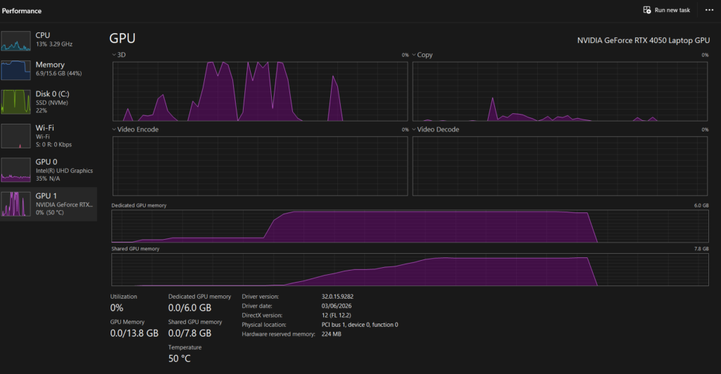
With rendering working, the default config (batch_size=25, train_res=512) ran out of memory on a 6 GB laptop GPU (RTX 4050) partway through the first step. The batch dimension and the render resolution both scale memory close to linearly, so both got reduced (batch_size=4, train_res=256) until a full 2,500-step run completed without OOM. This became the baseline configuration for every later experiment.
Swapping CLIP backbones without breaking assumptions baked into the code.
clip_model and consistency_clip_model are independently configurable, but the consistency-loss implementation (utilities/clip_spatial.py) hardcodes assumptions that only hold for the “Base” ViT variants: a for i in range(12) loop over transformer blocks (ViT-L/14 has 24), and an assertion that the patch stride evenly divides the patch size (ViT-L/14‘s 14px patch isn’t divisible by the default stride of 8, unlike 32px/16px). RN50 — a convolutional backbone — can’t be used for the consistency loss at all, since that code depends on ViT-style patch tokens that a ResNet simply doesn’t produce. ViT-B/32, ViT-B/16, and RN50 (as the primary loss only) were compared under an identical seed/mesh/prompt to keep the comparison controlled; ViT-B/32 was kept as the default going forward, primarily because it fit the VRAM budget without further code changes.
Debugging a mesh, not the code.
A custom tuna.obj mesh failed with CHOLMOD: not positive definite inside the Cholesky factorization. The Laplacian L is only positive-definite after pinning one null-space direction — which is correct for a single connected mesh, but insufficient if the mesh has multiple disconnected components (each contributes its own null direction). The tuna model’s eyes turned out to be separate, unwelded geometry. Diagnosing this required leaving the codebase entirely and going into Maya: using Mesh → Separate to count connected shells, Combine + Merge (vertex welding by distance) to attempt reattachment, and re-running Separate as the verification step (if it can no longer split the mesh, it’s genuinely one piece). Welding never fully closed the gap without visibly displacing the eyes during remeshing, so the pragmatic fix was deleting the eye geometry outright, producing tunaNoEyes.obj — a reminder that not every mesh bug is worth solving at the mesh level when the pipeline’s actual requirement (single connected component) can be satisfied more simply.
Stale caches and unattended runs.
MeshProcessor caches differential operators and Jacobian .npz files under <output_path>/tmp/ and silently reuses them if present — convenient for resuming, dangerous if the source mesh changes but the output path doesn’t: a later run against a re-exported (different vertex count) tuna.obj crashed in a sparse matrix multiply because the cached operators no longer matched. Once that class of bug was understood, a small driver script (run_batch.py) was written to chain multiple mesh/prompt runs sequentially — the single 6 GB GPU rules out any parallelism — each with a fresh output directory and its own log file, so a several-hour unattended batch could run overnight without one failed run silently corrupting the next.
Results
Five source→target pairs were run to completion on the final configuration (batch_size=4, train_res=256, ViT-B/32, single RTX 4050 Laptop GPU):
| Source → Target | Steps | Wall-clock |
|---|---|---|
cow → giraffe (spot.obj) | 5,000 | 1h 14m |
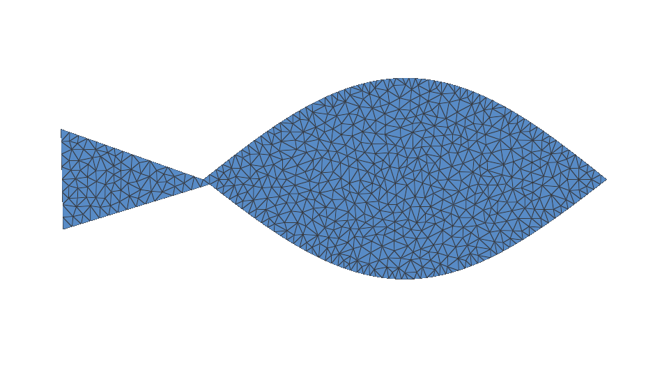
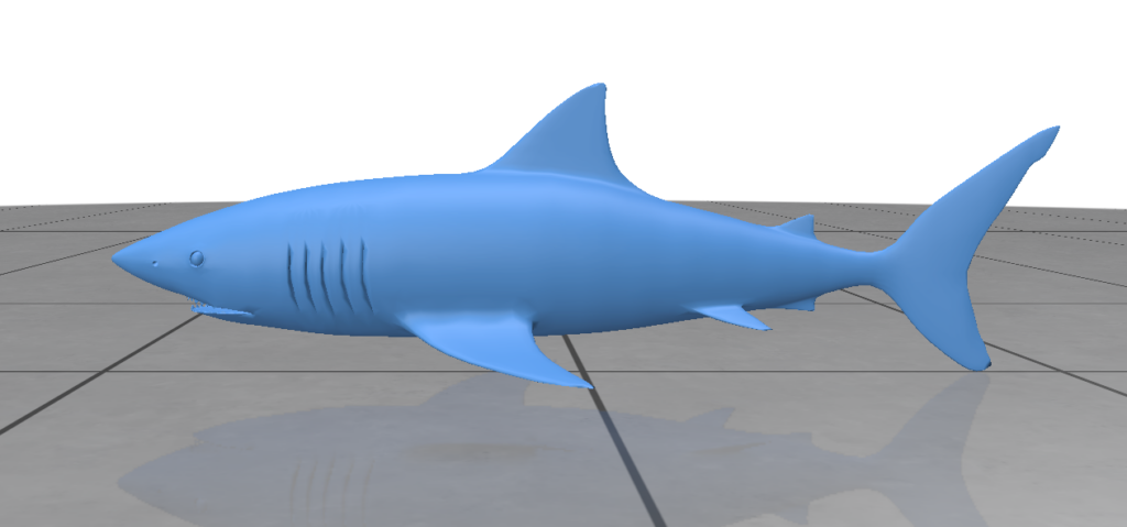
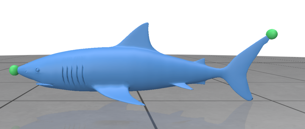
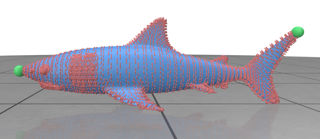
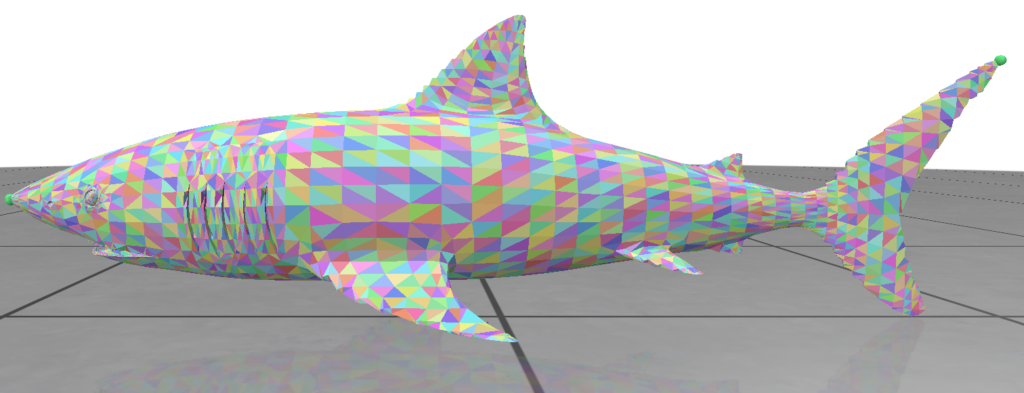
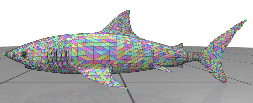
| fish → shark | 10,000 | 2h 37m |
| eiffel tower → rocket | 10,000 | 3h 21m |
tuna → shark (tunaNoEyes.obj, remeshed) | 10,000 | 2h 33m |
| guitar → axe | 600 | 9m 39s |
Per-step cost stayed in a fairly narrow band (~0.89–1.2 s/step) across meshes of similar triangle count, and scaled with batch_size × train_res as expected from the rendering cost analysis above — the guitar → axe run at 600 steps was deliberately short (~10 minutes) as a fast-iteration sanity check rather than a converged result, and looks correspondingly less refined than the 10k-step runs.
Future Work
Validate mesh topology before the Poisson solve, not during it.
The tuna.obj failure surfaced as a Cholesky exception deep inside training, three layers of traceback away from the actual cause (disconnected components). A pre-flight check — counting connected components with igl and failing fast with a clear message before any GPU work starts — would turn a confusing runtime crash into an immediate, actionable one, and is a small, self-contained addition to MeshProcessor.py.
Generalize the consistency-loss encoder beyond the “Base” ViT assumption.
The hardcoded 12-layer loop and stride-divisibility requirement in clip_spatial.py make ViT-L/14 unusable for the consistency loss without a code change, and rule out testing community-trained checkpoints (e.g. LAION’s ViT-B-32 retrained on LAION-2B via open_clip) that share the same architecture but arrive through a different loading path than OpenAI’s clip package. Both are architecture-family limitations, not fundamental ones — worth fixing before running a broader backbone ablation.
Reference
https://threedle.github.io/TextDeformer
ShapeFlow: Morphing Between 3D Shapes
We also explored a method for morphing one 3D shape into another target 3D shape. We worked with ShapeFlow, a neural network that learns to deform an existing 3D shape into another through a continuous flow field. Given latent space encodings of a source and target shape, the model outputs a velocity field describing how each point on the source should move to arrive at the target. Because the flow is continuous and (under the right conditions) bijective, the resulting deformation is guaranteed to be free of self-intersections, and can optionally preserve volume. Both of these properties can be desirable for artists working with meshes, which makes ShapeFlow attractive for toolification.
The Model
ShapeFlow’s creators frame the deformation of source shape into target shape as an advection process–the movement of a conserved property through fluid flow. Each point on the source is carried along a flow field over an interpolation parameter . Then, the points of the deformed source shape are described as:
Training seeks the mapping that minimizes the symmetric Chamfer distance between the deformed source and the target:
So the output of ShapeFlow is this flow field or mapping that describes how each point on the source shape should advect in order for the source to become the target shape. How are the inputs to ShapeFlow created? What do we feed to the model?
Recall, we said that the input to ShapeFlow is the pair of latent space encodings from the source and target shapes. For our implementation, we use an encoder that maps a mesh’s vertices to a latent space encoding using a single forward pass. The encoder is trained jointly with the deformer model, using the same Chamfer distance loss, so it learns to produce encodings that are useful for conditioning the flow field.
The Toolification
Our goal was to implement ShapeFlow as a Maya plug-in for artists’ use in stylization and retopology of one mesh to another. To increase usability, we added blendshapes between the source mesh and the deformed source mesh by extracting and exporting intermediate results along the deformation path (sampling at intermediate values of ). This way, an artist can scrub through the flow and select whichever stage best fits their needs.
Future Exploration & Improvement
While implementing ShapeFlow as a Maya tool for artists, we ran into some areas of exploration for the performance of the tool. With more time we would have done more experimenting and development to ensure the model’s capabilities are consistent and high-performing for our desired use cases. On the SGI timeline we ultimately decided to balance exploration and execution and forge ahead with building out the tool while noting areas for improvement:
- Initialization Sensitivity: Since the initialization of the model weights are random, results can vary widely based on whether one initialization was “good” for the specific meshes being used.
- Loss Function Limitations: One of the use cases we wanted to develop ShapeFlow for was to create intermediate expressions for a given face mesh with certain extreme expressions. However, when morphing between meshes that differ only in a small region–for example puckered lips vs. a neutral expression–the region may be too small to affect the Chamfer distance loss during optimization. Other loss functions are worth evaluating for these cases.
- Pretraining: If there are certain use cases (classes of objects, faces) that ShapeFlow will be used for, it might be beneficial to do pretraining on those types of shapes. Currently, our tool trains the deformer model from scratch every time. (This is also why the initialization sensitivity affects the results so strongly.) As a result, the model either will take an extremely long time with an appropriate amount of training iterations, or be used after a lower number of training iterations with reduced fidelity.
We did some manual tuning to get workable results on our test meshes, but making this robust enough for an artist’s workflow requires additional experimentation, testing, and development.
Results
Below is a video demonstrating the Maya tool workflow. For the sake of time, in the video the model is only trained for 200 iterations (very low), which is one source of the poor or unfinished-looking output flow.
Below is an image showing how ShapeFlow can be used to produce a blend of two meshes. The ShapeFlow output (middle) is result of Toilet 1 (left) morphing into toilet 2 (right).