Have you ever tried moving a sofa through a narrow staircase? Every twist, turn, and pivot matters, and one wrong angle means you’re stuck. In robotics and computational geometry, this is famously known as the “Piano Mover’s Problem.”
But what if the “piano” is a highly intricate, symmetrically interlocked mathematical sculpture?
For my project, I decided to tackle the challenge of computationally disassembling the beautiful, mind-bending geometric sculptures designed by George Hart.

To do this, I built a motion planning pipeline using the Open Motion Planning Library (OMPL) to find collision-free paths, Polyscope to visualize the 3D physical world, and Matplotlib to peek into the “brain” of the algorithm by plotting the 2D Configuration Space (C-Space).
Let’s dive into how we can use geometry to escape the cage, navigate the galaxy, and eventually… get completely snarled.
The Setup: Workspace vs. Configuration Space
To disassemble these symmetric sculptures, all identical pieces must move away from the center simultaneously. To simplify our problem, we define our state by a translation displacement “d” and a local rotation. While our algorithm supports rotation in “x”, “y”, and “z”, we found that moving outward with respect to the origin and rotating around the Z-axis is often the key to unlocking these puzzles.
This gives us two very different ways to look at the same problem:
The C-Space (Matplotlib): The Configuration Space is a theoretical space where the entire sculpture is represented as a single point. I used Matplotlib to take 2D slices of this space (Displacement “d” vs. Rotation in Z). We evaluate thousands of states using the FCL (Flexible Collision Library). If a state has overlapping meshes, we color it red (Collision). If it’s safe, we color it green (Free Space).
The Workspace (Polyscope): This is the 3D physical space where the meshes actually exist and move. It’s what we see with our eyes.
The Algorithm: Growing Trees with OMPL
To find a valid path from the assembled state (Start) to the fully separated state (Goal), I used RRT-Connect from OMPL.
Imagine two vines growing blindly—one from the Start state and one from the Goal state. They branch out randomly into the free space of our C-Space, hoping to eventually touch and connect.
RRT-Connect is incredibly fast in wide-open spaces. However, it has a famous Achilles’ heel: The Narrow Passage Problem. If the only way to solve a puzzle is through a tiny, precise series of movements, the random vines have a very low probability of growing exactly into that microscopic corridor.
To test this, I ran the planner on three different George Hart sculptures. Here is what happened.
Experiment 1: Cagework (The Walk in the Park)
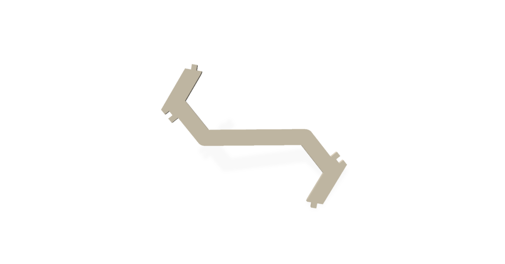
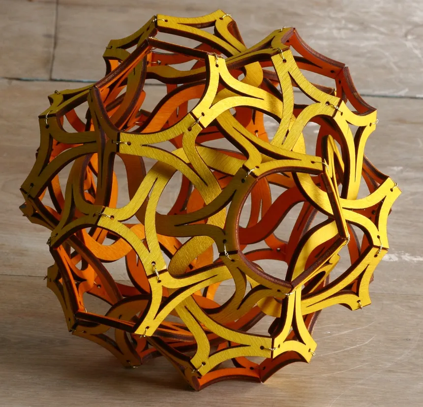
We started with Cagework. In the physical world, it looks like a complex cage of intersecting edges. But what does the algorithm see?
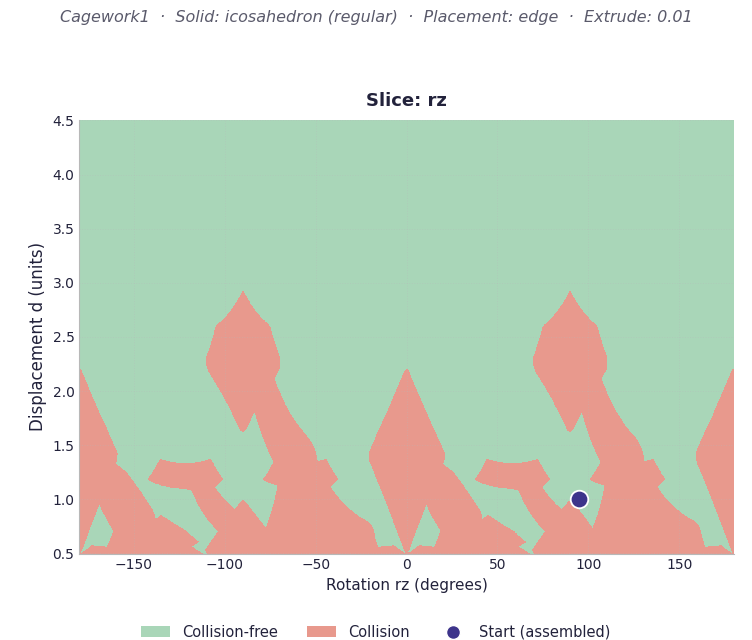
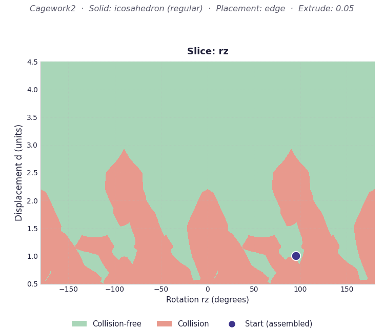
Because the C-Space has wide, forgiving green areas, our RRT-Connect algorithm has no trouble finding a path. Any random sample is likely to fall in a valid state.
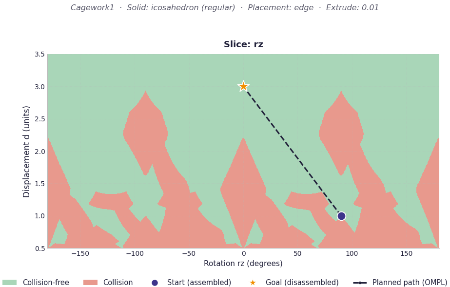
The result in the workspace is a smooth, immediate disassembly.
Experiment 2: Galaxy (The Narrow Passage)
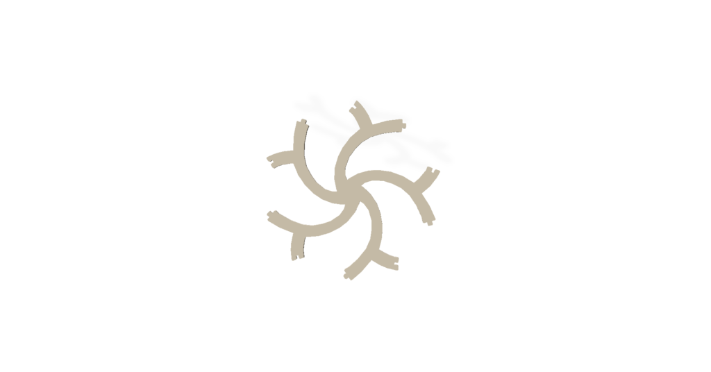
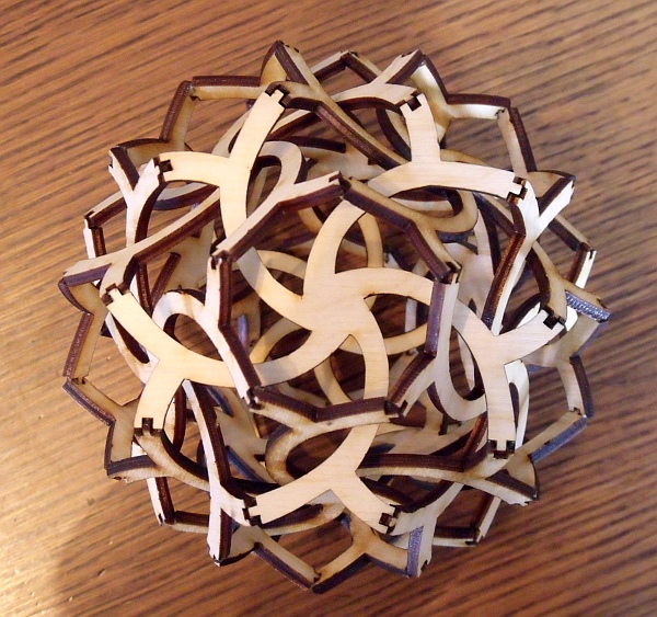
Next, we tried Galaxy. This is where things got interesting. The pieces are much more tightly packed, requiring a very specific twisting motion to separate.
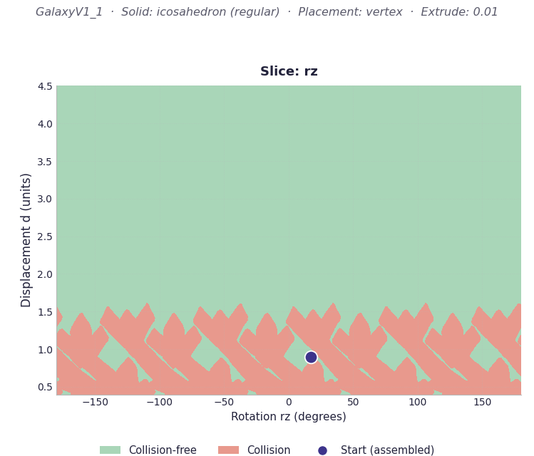
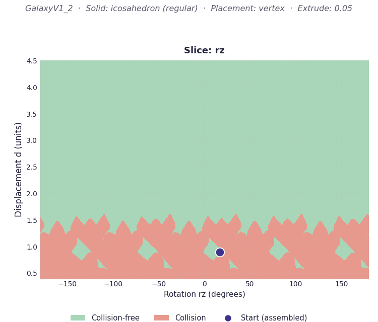
This is a classic narrow passage. OMPL’s RRT-Connect had to work much harder here. The algorithm threw thousands of random branches, most of them hitting the red “collision” walls, until one lucky branch managed to thread the needle through the bottleneck.
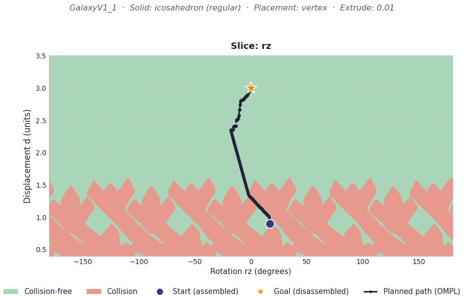
When we animate the OMPL path in Polyscope, you can see exactly why this was so hard: the pieces barely scrape past each other, requiring a perfectly timed Z-rotation paired with the outward displacement.
Experiment 3: Snarl (The Impossible Snag)
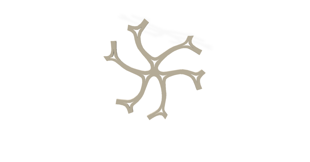
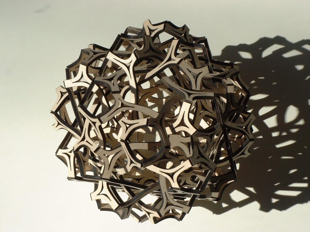
Finally, we tested Snarl. As the name implies, this sculpture is a geometric knot. I set up the planner, hit run, and… nothing. The planner timed out. Instead of staring at a blank screen, we can use our Matplotlib C-Space plots to diagnose why it failed.
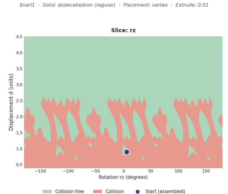
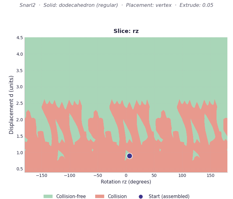
The 2D C-Space slice tells the whole story. The green space is completely disconnected, or the required passage is so microscopically narrow that it falls below our collision_tolerance (0.0001) and state_validity_resolution. The vines of our RRT-Connect were trapped in a cage of collisions, unable to reach the goal.
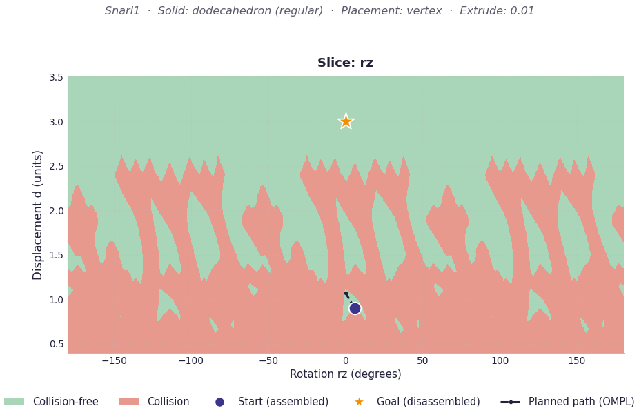
While a pure symmetrical displacement + rotation couldn’t solve Snarl, this “failure” is actually a success in visualization. It proves that the topology of the sculpture inherently locks itself in place under these symmetric constraints!
Conclusion & Future Work
Working on this project was a fantastic journey into how robots “think” about space. What looks like a physical interlocking puzzle to us is just a maze of high-dimensional obstacles to an algorithm.
By bridging OMPL, Polyscope, and Matplotlib, I learned that:
- Visualization is debugging: I wouldn’t have understood why Snarl failed without plotting the C-Space.
- Topology dictates performance: An algorithm is only as fast as the width of its narrowest passage.
In the future, it would be fascinating to expand the Matplotlib visualization to 3D slices (adding Rx or Ry into the mix) to see if Snarl has a hidden escape route in higher dimensions, or to implement path smoothing to make the Galaxy disassembly look less erratic.
A huge thank you to the SGI mentors and the amazing community for this experience!
