Mentor(s): Dr. Ahmed Mahmoud [MIT], Ana Dodik [MIT]
Fellow(s): Gokul Adithya Suresh [RVCE], Yufan (Diana) Hu [Macalester College]
Volunteer: Ruyu Yan [Princeton University]
Introduction
When we think about the shortest path between two points, we usually imagine a straight line (a Euclidean distance). But once those points lie on a curved surface, the notion of a straight line becomes more subtle. The shortest path must follow the geometry of the surface itself. Such paths are called geodesics.
Geodesics are fundamental to understanding how geometry shapes motion and distance. Given a surface, we can ask where its geodesics go, how far apart points are, and how the geometry influences the paths between them. This is the familiar forward perspective: given the geometry, determine the resulting geodesic structure.
But what if we reverse the question?
Instead of starting with a surface and asking what paths it produces, we can start with a desired path or geodesic behavior and ask what geometry would produce it. This shift, from computing geodesics on a given surface to designing the surface around desired geodesics, is the central idea of inverse geodesic design.
At its core, inverse geodesic design is therefore a problem of shaping geometry through the behavior it induces. By modifying the surface, we modify its intrinsic metric, which in turn changes its geodesic distances and paths. The challenge is to find a geometry whose geodesic structure matches a desired objective.
This simple reversal opens up an interesting computational problem: can we design a surface by optimizing it directly through its geodesics?
Geodesics with the Heat Method
To design a surface around its geodesics, we first need to measure geodesic distance on a mesh, and measure it in a way we can differentiate later on. We use the Heat Method for this (Crane, Weischedel and Wardetzky, 2013).
The idea goes back to an observation by Varadhan. Put a spot of heat at a point, let it diffuse for a very short time, and the way it spreads already tells you how far away everything is. Nearby points warm up fast, far points stay cold. The Heat Method takes this and turns it into three steps, and each one is just a sparse linear solve. That last part is what we care about, since it means we can differentiate through the whole thing.
Step 1: Diffuse heat from the source
We place a unit heat source on the source set and let it spread for a short time . In discrete form this is a single backward-Euler step of the heat equation:
where is the cotangent Laplacian, is the (lumped) mass matrix, and marks the source vertices. Solving this gives , a smooth blob of heat sitting around the source.
Step 2: Normalize the heat gradient
The gradient of the heat field points away from the source, which is the direction distance grows in. Its length is not useful to us, since the heat fades as you move away, but its direction is exactly what we want, so we normalize it to a unit vector field:
The minus sign makes point away from the source. This gives us a good guess for which way the real distance function should be increasing at each point.
Step 3: Recover distance with a Poisson solve
The last step is to find a scalar field whose gradient lines up with as closely as it can. That is a Poisson equation:
and then we shift so it reads zero at the source. What comes out is the geodesic distance, up to the usual approximation, from to every vertex.
The time sets how much the field gets smoothed. We use with the mean edge length and across all our grids. Since the three steps are all sparse solves, comes out as a differentiable function of the vertex positions. In iskra this is one call, heat_method_distance(V, F, src), and we drop it straight into the optimization loop so the gradients can flow back through it.
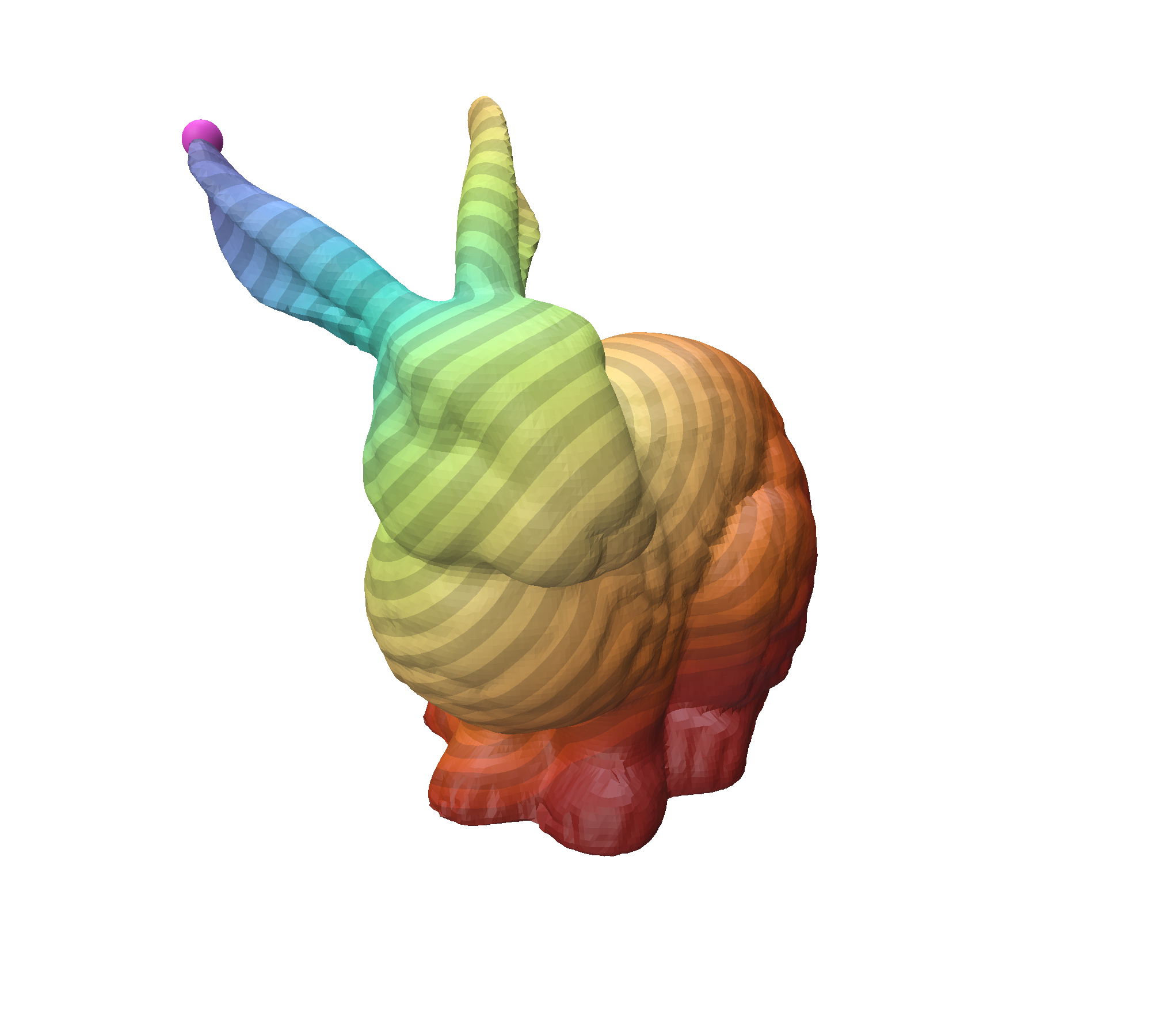
This is the Heat Method on a real 3D mesh. We put one source on the bunny’s ear and colour each vertex by its geodesic distance from it, so every band is a ring of equal distance. The bands wrap around the ears and body instead of cutting straight across, which is the surface geometry bending the distances. Later we deform a surface on purpose to control exactly this.
Building Geometric Intuition
Formulas are easier to believe once you can poke at them and watch what happens. So we built a small interactive demo in Polyscope for the forward problem, the one we have been describing so far.
Forward: distance follows the geometry
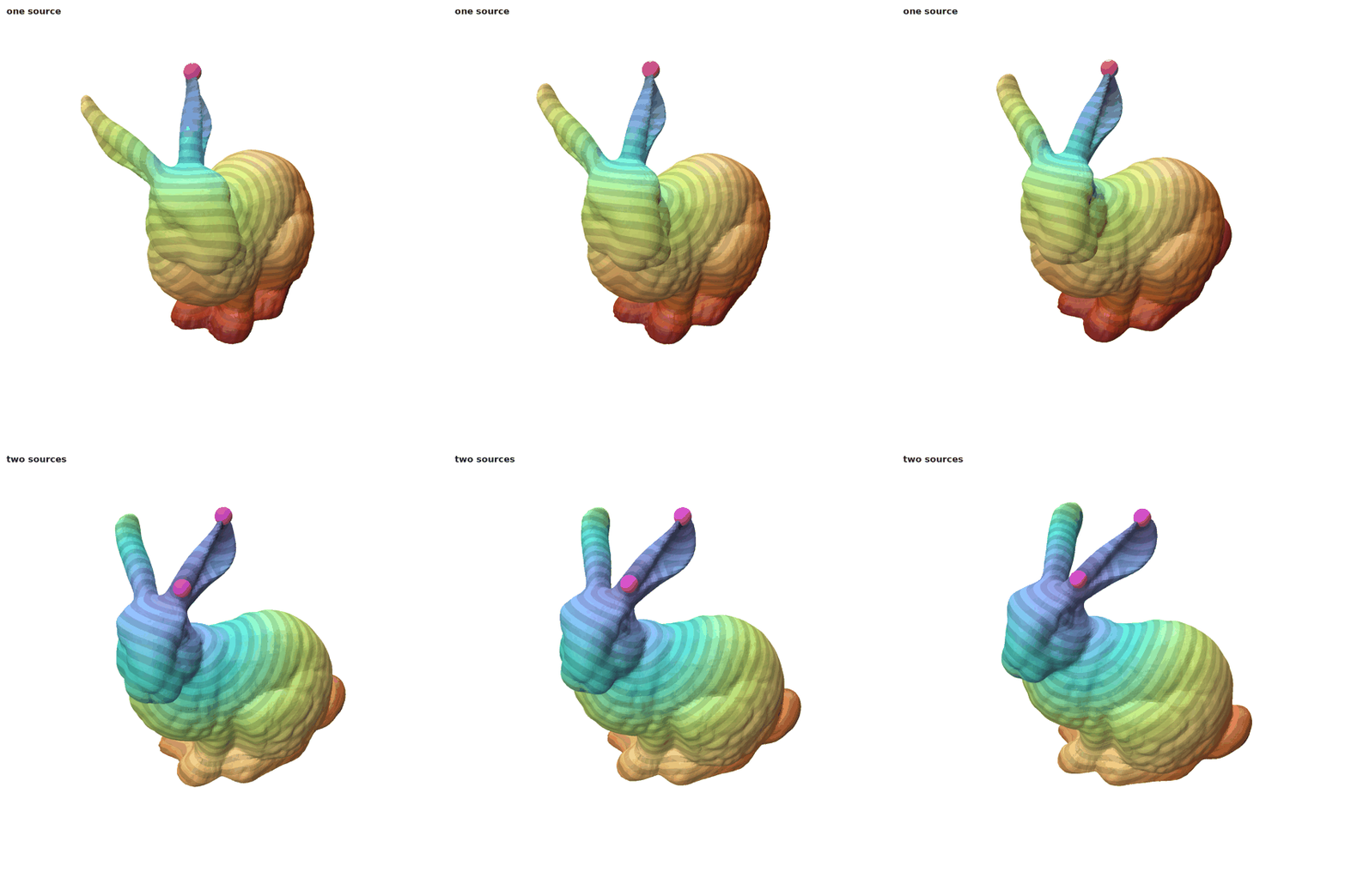
In the forward demo you click a source vertex and the distance field and its isolines redraw live. On a flat sheet the contours come out as neat circles. Bend the surface into hills and valleys and they start to stretch and bunch up, since the shortest path now has to climb over or go around whatever is in the way. This is the idea the whole project sits on: the shape of the surface is what sets the distances.
You drop a source and the distance field shows up right away. We start with one source, then add a second, and the field redraws. Each point just takes the distance to the nearer source, so a line forms where the two regions meet.
Inverse Geodesics
So far we have only read distances off a fixed surface. The inverse problem turns that around. We decide where the source and the target points sit and what distance we want between them, and then we let the surface itself change until that is true. Nothing about the layout moves, only the heights, so the terrain rises and dips until the geodesic distance to the target lands where we asked. The rest of this section makes that concrete: how we set up the terrain, what we minimize, and how we keep the surface from turning into noise.
Problem Formulation
For our experiments, we keep the setup clean. We represent the terrain as a triangular heightfield over the plane. The planar coordinates and mesh connectivity remain fixed, while the vertex heights (y – coordinates) are optimized.
Given a source set and target set , our goal is to deform the surface until every vertex in has approximately the same geodesic distance from .
For the examples here, we pick a grid diagonal as our target, though in practice can be any arbitrary subsets of vertices you want to align.
Distance Objective and Optimization Workflow
We measure the geodesic distance at every vertex using the differentiable Heat Method. Let be the target vertex set and let be the desired geodesic distance from the source set. We define the distance loss as
In plain terms, this asks every target vertex to sit at the same chosen distance from the source, and it grows whenever one of them drifts off that distance.
We optimize the mean squared distance error and report its square root,
which has the same units as geodesic distance.
We optimize the vertex heights using Adam over a fixed number of iterations. Each iteration follows this pipeline:
Vertex heights
↓
Construct the heightfield mesh
↓
Compute Heat Method distances
↓
Evaluate
↓
Compute height gradients with backpropagation
↓
Update vertex heights with Adam
↓
Repeat until the final iteration
Since the Heat Method implementation is differentiable, the gradient of can be computed with respect to the vertex heights. We initialize the surface with a small sinusoidal perturbation (amplitude ) to break initial planarity without introducing high-frequency noise.
Baseline: Distance Loss Only
We first optimized the heightfield using only the distance objective, that is, with the smoothness weight set to zero (we introduce that term in the next section):
The optimization reduces the on , making the target diagonal approximately follow a geodesic-distance contour.

The red points are the target vertices, and the yellow curve is the desired distance contour ().

While minimizing successfully aligns the target distance, it places no constraint on local surface geometry. Therefore, a small distance loss can still produce high-frequency surface noise and localized spiky oscillations.
Regularizing the Surface
To enforce smoothness on the optimized surface, we consider two regularization schemes: height smoothness and normal smoothness.
We first penalize height differences between neighboring vertices. Let be the set of horizontal and vertical grid edges, and let be the height of vertex . We define the height smoothness as,
The loss is small when neighboring vertices have similar heights and large when their height difference increases. Then, the complete objective is
Height smoothness directly controls neighboring height differences. However, it does not directly measure changes in triangle orientation. A surface can therefore have relatively small height differences while still containing visible local bends.
To fix this, we switch to Normal Smoothness, which penalizes orientation changes between adjacent face normals rather than absolute height differences. For each adjacent face pair , let and be their unit normals.
The final objective is
Pareto Analysis for Smoothness-Weight Selection
The regularization weight dictates the trade-off between geodesic target fidelity and surface smoothness. To select more reasonable optimal hyperparameter values, we sweep and construct Pareto frontiers plotting RMSE against and , respectively.
For height regularization, each point is plotted as
and for normal regularization as
Both coordinates are minimized. A point is Pareto-optimal if no other run achieves both lower RMSE and lower smoothness energy.


These plots are used independently because the two smoothness energies have different meanings and scales. For each regularizer, we choose a weight near the knee of its Pareto curve: the point beyond which further smoothing causes a much larger increase in distance error.
Visual Comparison
Based on the Pareto curves, we select one representative weight for each regularizer and rerun the optimization to visualize the resulting terrains. Both experiments use the same source, target vertices, desired distance, and initial heightfield.
- Set for height regularization


It produces several sharp folds and zigzag-like oscillations near the target set. It controls neighboring height differences but does not directly constrain changes in face orientation.
- Set for normal regularization


Normal regularization produces a smoother and more coherent terrain. The deformation is distributed gradually around the target set, forming a continuous ridge without the sharp folds and zigzag-like oscillations observed under height regularization. This reflects the direct penalty on orientation changes between adjacent faces.
The corresponding measurements are summarized below.
| Metric | Height regularization | Normal regularization |
| Target-distance RMSE | ||
| Maximum target error | ||
| Target-distance range | ||
| Height smoothness | ||
| Normal smoothness | ||
| Height range |
Remark: Our main goal is to remove noisy folds and produce a smoother terrain. Normal regularization achieves this more effectively by directly penalizing orientation changes between adjacent faces. We therefore use normal smoothness in the following experiments.
Forward Solver Comparison: Convex RGD vs. Heat Method
iskra’s original code computes the forward distance field with a convex-optimization solver, following the regularized geodesic distance (RGD) formulation of Edelstein et al., solved with an ADMM scheme. We compare that convex solver against the Heat Method while keeping the inverse optimization setup fixed.
Both methods use the same grid, source, target vertices, desired distance, stopping tolerance, and maximum number of iterations. Each experiment is repeated five times.
| Forward solver | Converged runs | Iterations | Median time | Final L2 error | Final RMSE | Max error |
|---|---|---|---|---|---|---|
| Convex RGD (Edelstein et al.) | 0/5 | 50 | 59.41 s | 0.1307 | 0.0394 | 0.0694 |
| Heat Method | 5/5 | 29 | 3.97 s | 0.00948 | 0.00286 | 0.00575 |
Across all test runs, the Heat Method converges in all five runs and is approximately 15 times faster than the convex RGD solver. It also reaches a substantially lower distance error. We therefore use the Heat Method as the forward solver in the following experiments.
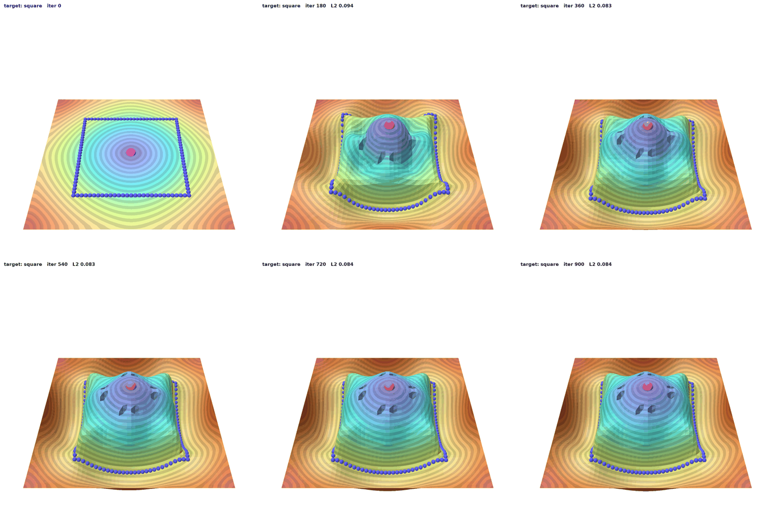
Before moving on, here is the whole thing running. We fix a target outline and a distance, and the flat sheet bends frame by frame until the geodesic contour traces the shape we asked for. The source ends up on top and the contours run downhill into the target.
Going Neural: Terrain as an MLP
Up to this point the unknowns were the vertex heights themselves, one number per vertex. In week 6 we swapped that out. Instead of keeping a separate height at every vertex, we let a small neural network hand us the height as a continuous function of position:
and we optimize the network weights rather than the heights. The rest of the loop does not change at all. We build the mesh from these heights, run the Heat Method, measure the distance loss, and take an optimizer step. The one thing that is different is where the heights come from.
There are a few reasons to do this. The network is defined everywhere on the domain, not only at the grid points, so it does not really care about the mesh resolution and we can train on a coarse grid and then read it off on a finer one. It also comes out smooth on its own, and the parameter count stays fixed no matter how many vertices we throw at it.
Implementation
The height field is a small multilayer perceptron. It takes the coordinate pair , normalized to , runs it through two hidden layers of width 64 with activations, and returns a single number. We squash that output so the heights cannot run off to anything extreme:
Here is a height cap, setting how far up or down the terrain is allowed to go. The whole thing still sits on top of iskra’s differentiable Heat Method, so the gradient from the distance loss makes it all the way back to the weights . The loop now looks like this:
Network weights θ
↓
Heights yi = fθ(xi, zi)
↓
Construct the heightfield mesh
↓
Compute Heat Method distances
↓
Evaluate Ldistance
↓
Update θ with Adam
Preliminary visuals based on MLP
To validate implicit neural representations for terrain design, we fit a coordinate-based MLP on a coarse grid. The network converges after iterations in seconds. The final target-distance RMSE is , with a maximum target error of .

After training, we evaluate the same MLP on a finer grid without further optimization. This coarse-to-fine evaluation produces a denser visualization of the learned continuous heightfield while preserving the height range .

The finer sampling shows that the learned terrain remains continuous across resolutions and that the target set closely follows the desired distance contour.
Effect of Output Scale and Activation Function
The MLP output scale limits how much the terrain can deform. When the scale is too small, the network cannot produce enough height variation to match the target distance.
| Scale | Converged | Iterations | RMSE | Normal smoothness | Height range | Runtime |
|---|---|---|---|---|---|---|
| 0.05 | No | 400 | 0.2935 | 0 | 0 | 30.54 s |
| 0.10 | No | 400 | 0.1432 | 0.00689 | 0.200 | 30.17 s |
| 0.15 | No | 400 | 0.0678 | 0.00866 | 0.300 | 30.91 s |
| 0.20 | Yes | 27 | 0.0317 | 0.00241 | 0.400 | 2.13 s |
| 0.25 | Yes | 21 | 0.0303 | 0.00092 | 0.443 | 1.66 s |
| 0.30 | Yes | 18 | 0.0289 | 0.00079 | 0.505 | 1.40 s |
| 0.40 | Yes | 14 | 0.0315 | 0.00063 | 0.543 | 1.10 s |
The optimization fails to converge for scales below . At these scales, the learned height range reaches the available output range, indicating that the MLP does not have enough vertical freedom. For the following experiments, we use scale =
We also compare several activation functions across five random seeds. The seed controls the initial values of the network parameters. Repeating each experiment with multiple seeds therefore measures the stability of each activation rather than relying on a single favorable run.
| Activation | Convergence rate | Median iterations | Median RMSE | Median normal smoothness | Median runtime |
| Tanh | 0.80 | 30 | 0.0369 | 0.00255 | 2.39 s |
| ReLU | 1.00 | 30 | 0.0307 | 0.00311 | 2.33 s |
| Softplus | 1.00 | 56 | 0.0294 | 0.00350 | 4.37 s |
| SiLU | 1.00 | 39 | 0.0336 | 0.00235 | 3.05 s |
No single activation function performs best across all metrics. ReLU provides the lowest median runtime, Softplus achieves the lowest median RMSE, and SiLU produces the lowest median normal-smoothness energy. Tanh is less robust, with one run failing to converge.
Consequently, this is a full multi-objective comparison that could use Pareto analysis to balance accuracy, smoothness, runtime, and convergence stability. We leave this analysis for future work and use Tanh as a fixed activation function in the following experiments
Fourier Analysis of the Plain MLP Heightfield
Before introducing positional encoding, we first examine the frequencies represented by the plain coordinate-based MLP. Since the learned terrain is a continuous function , we can decompose its sampled heightfield into a spatial frequency components.
This analysis shows whether the learned surface is dominated by broad, long-wavelength deformation or also contains shorter-wavelength local detail. It also provides a baseline for evaluating how positional encoding changes the frequency content of the terrain.
We sample the trained MLP on an grid and denote the resulting heights by . Before computing the Fourier transform, we remove the mean height,
This removes the constant vertical offset and leaves only spatial variation. The Fourier coefficients are
with power,
After shifting the zero-frequency coefficient to the center, coefficients near the center describe broad terrain deformation, while coefficients farther away describe finer spatial variation. We display .
To obtain the radial power spectrum, we group the coefficients by normalized radial frequency,
where and are the frequencies along the x – and z – directions. We then average the power of coefficients with similar radial frequencies. This removes directional information and shows how the spectral power changes with overall frequency magnitude.
To compare broad deformation with finer geometric variation, we divide the normalized frequency range at :
This cutoff separates the region near the frequency origin from the higher-frequency portion of the spectrum.

The 2D log-power spectrum (left); radial power spectrum (right). The dashed line marks the normalized frequency cutoff at (0.25).
The radial power decreases rapidly with frequency. Nearly all spectral power lies below the cutoff, while the high-frequency contribution rounds to . This shows that the learned terrain is dominated by large-scale, low-frequency deformation.
So what does this tell us for the inverse problem? The plain MLP hits its distance targets almost entirely through broad, large-scale deformation rather than fine local adjustments, which is why the surface stays free of vertex-level noise even while moving large regions of the terrain. The analysis does not change the geometry itself; it pins down the limitation of this representation, that it has essentially no high-frequency content, and that is exactly what motivates positional encoding, which we turn to next to add short-wavelength detail when a target needs it.
The Fix: Positional Encoding
The plain MLP has a built-in weakness known as spectral bias. Networks pick up smooth, low-frequency shapes almost immediately, but sharp, high-frequency detail comes very slowly, if it comes at all. So when the target we want has sharp features, like corners or a thin ridge, the plain MLP barely budges. There is almost no gradient pushing it toward that high-frequency shape, and it just stays smooth and flat and never gets near the target.
The fix is positional encoding. Instead of handing the network the raw coordinates and waiting for it to build high frequencies by itself (it will not), we give it those frequencies up front. Before the MLP sees anything, we expand each coordinate into a set of sinusoids at rising frequencies:
and feed this encoded vector to the same MLP:
Now that the high frequencies are already sitting in the input, the network does not have to conjure them up, and it can actually draw sharp terrain. The number of bands is the only real knob here, and more bands buys you finer detail. We build with iskra’s HarmonicEmbedding, so none of this adds any extra learnable parameters.
Result 1: sharper contours for the same budget
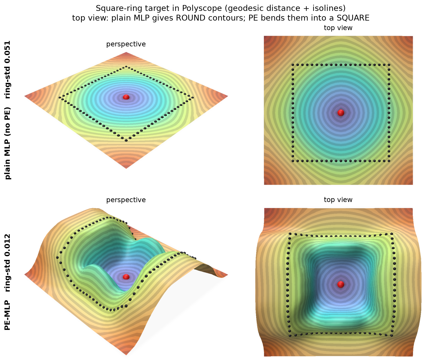
With the same height cap and the same training budget, the plain MLP gives us round, washed-out contours, while the positional-encoding one actually lands on the sharp target shape we asked for. The top-down view is where the gap really shows.
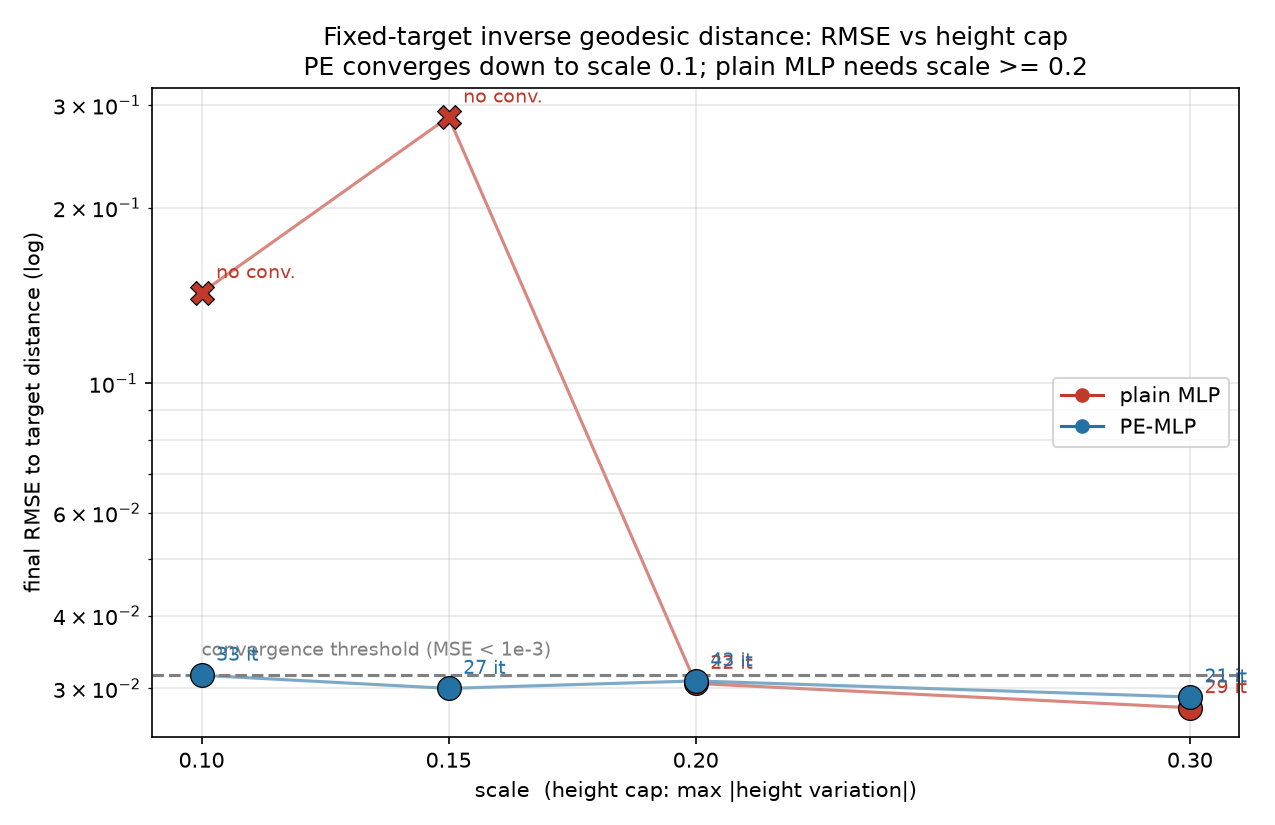
Result 2: the target at a smaller height budget
We also swept the height cap directly. As we shrink , the terrain has less room to move, so reaching the target distance gets harder. The positional-encoding MLP still converges all the way down to scale 0.1, whereas the plain MLP gives up somewhere below 0.2. So positional encoding gets to the same target on roughly half the height budget.
Future work
What is next: MLP-derivative smoothness
Since the terrain is now a proper continuous function, the smoothness question gets cleaner. The mesh-based terms we used earlier, penalizing height differences between neighbors or the bending between adjacent face normals, are really measuring one particular triangulation. Refine the mesh and the same surface gives a different penalty, which always felt slightly off, since what we actually care about is whether the underlying surface is smooth. With the MLP we can ask that directly. Because the height is a differentiable function of position, we hand the coordinates to autograd, get the true gradient of the surface at any point, and penalize its magnitude:
Unlike the mesh-based smoothness terms, this one does not depend on the mesh at all. It reads the smoothness of the surface itself, so training on a coarse grid and evaluating on a fine one gives a consistent notion of smooth either way. The next step is to run the same accuracy-versus-smoothness sweep we did for the mesh terms, but with this derivative penalty, and see where it lands on the trade-off curve. Our hunch is that it gives a gentler, more uniform surface for the same distance error, since it is not chasing per-triangle artifacts.
A couple of other directions we want to chase from here:
- Bringing surface normals into the objective. Regularizing or matching normals, rather than only distances, is a natural next lever and something our smoothness experiments already hinted at.
- Scaling to many sources and harder targets. Our tests so far used one or two sources and fairly simple contours. Pushing to many sources and genuinely complex target shapes is where the positional-encoding advantage should matter most.
- Combining positional encoding with the derivative smoothness. The two ideas are independent, so pairing them should give sharp targets on a clean, mesh-independent surface.
Reference
- Edelstein, M., Guillen, N., Solomon, J., and Ben-Chen, M. “A Convex Optimization Framework for Regularized Geodesic Distances.” SIGGRAPH 2023 Conference Proceedings, 2023. https://doi.org/10.1145/3588432.3591523
- Dodik, A., Mahmoud, A. H., and Solomon, J. “Iskra: A System for Inverse Geometry Processing.” 2026. https://arxiv.org/abs/2602.12105
- Iskra source code: https://github.com/anadodik/iskra
