Approximate 3D Convex Decomposition

By Gizem Altintas, Biruk Abere Ambaw, Francheska Kovacevic, Emi Neuwalder

During the first week of SGI, we worked with Prof. Yusuf Sahillioglu and Devin Horsman to explore convex geometry and some of the 3D decomposition techniques.

1.     Introduction:

3D convex decomposition refers to a computational technique that breaks down a 3D object (usually represented as a mesh) into smaller convex sub-components. It is a popular computational process in computer graphics, computational geometry, and physics simulations. In other words, the objective of a 3D convex decomposition is to divide a complicated 3D object into a collection of simpler, non-overlapping convex shapes (convex polyhedra). These convex shapes are simpler to work with for a variety of tasks, including volume calculations, collision detection in physics simulations, and optimization in computer-aided design and modeling. An approximate convex decomposition aims to decompose the 3D shape into a set of almost convex components, which allows for efficient geometry processing algorithms, since computing an exact convex decomposition is an NP-hard problem.

2.      Work:

2.1.   Understanding Concavity Measurement

Our task was to identify concavity and observe some measurements in a mesh. We followed two different approaches using Dihedral Angles and Qhull.

Before diving into the methods, let us define what is a convex surface and a convex edge.

A convex surface is a type of surface in geometry that curves outward, like the exterior of a sphere or a simple convex lens. It is a surface where any two points on the surface can be connected by a line segment that lies entirely within or on the surface itself. In other words, a line segment drawn between any two points on a convex surface will not cross or go inside the surface.

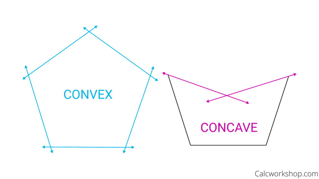
Fig.1: Some visualization for convexity

A convex edge is a type of edge that is part of a convex surface or shape. It is an edge where the surface or shape curves outward, away from the observer, along the entire length of the edge. For example, in Fig.1, all the edges in the left polygon are convex, while the interior edges with pink coloring on the right polygon are not.

A concave shape is characterized by at least one region or part that curves inward, creating an indentation or hollow area. It has sections that are “caved in” or indented. They can have complex curvatures and may require additional consideration in calculations and analysis.

Understanding the difference between convex and concave shapes is important in geometry and various fields such as computer graphics, physics, and design. Convex shapes are often preferred for their simplicity and ease of analysis, while concave shapes offer more intricate and varied forms that can be utilized creatively.

2.1.1.   Dihedral Angles

A dihedral angle is the angle between two intersecting planes or half-planes.

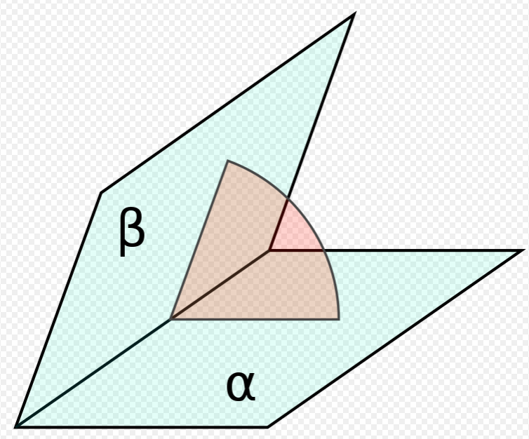
Fig.2: Dihedral angle between two half-planes (α, β, pale blue) in a third plane (red) which cuts the line of intersection at right angles

To determine which edges in the mesh exhibit concavity with dihedral angles, we followed a step-by-step process:

1. Compute unit normals per triangle:

Calculate the unit normal vectors for each triangle in the mesh. The unit normal represents the direction perpendicular to the surface of each triangle.

2. Compute the sine of the interior angles:

Since the calculated dihedral angles between two normals of triangles are treated as inner angles by our calculation. They were always between (0,180). We realized we needed a sign to differentiate between them. After searching, we found that:

A polygon with n vertices, p₁,…,p_n, is considered convex if, when its vertices are considered cyclically (with p₁=p_n), the cross products of consecutive edges,bi=(pi-pi-1) (pi+1-pi), all have the same sign or are zero. This means that the sine of the interior angles at each vertex, θ_i, has the same sign. If all sinθ_i are nonnegative or all nonpositive, the interior angles are at most 180°, indicating a convex polygon. If all sinθ_i are positive or all negative, the interior angles are strictly less than 180°, also indicating a convex polygon. This method allows determining polygon convexity without needing to check every angle explicitly, exploiting the properties of the sine changing sign for angles less than zero or greater than 180°.

In a formulated way, if n_a and n_b are the normals of the two adjacent faces, and p_a and p_b vertices of the two faces that are not connected to the edge, wherein n_a and p_a belong to the face A, and n_b and p_b to the face B, then

( p_b – p_a ) . n_a <= 0 => ridge edge

( p_b – p_a ) . n_a > 0 => valley edge

(Source)

3. Compute the dihedral angle between two triangles:

Determine the angle between the unit normals of two triangles that share an edge. This angle represents the deviation between the neighboring triangles indicates concavity degree. When the angle is close to 180 degree, we behave this edge as convex.

By following these steps and applying them to the given mesh, we were able to identify the concave edges. The result is a set of edges that exhibit concavity, which can be further analyzed or utilized for the intended purpose.

Here are some visualizations: For visualization, we have utilized Coin3D which is an OpenGL-based, 3D graphics library.

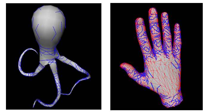
Fig.3: Our result with detected concave edges (marked with blue). For the hand model on the right, the red edges are convex edges whereas blue edges are concave.

The OFF files are from the following: Xiaobai Chen, Aleksey Golovinskiy, and Thomas Funkhouser, (A Benchmark for 3D Mesh Segmentation)[https://segeval.cs.princeton.edu/public/paper.pdf] ACM Transactions on Graphics (Proc. SIGGRAPH), 28(3), 2009. [(BibTex)[https://segeval.cs.princeton.edu/public/bibtex.html]]

2.1.2.   Concavity Measurement in 3D Meshes using Qhull

This method involves collecting triangles that share specific edges, creating a point set from these triangles, and then calculating the difference between the point set and its convex hull. Through this exploration, we sought to understand the significance and applications of this novel concavity measure using Qhull for analyzing 3D meshes. 

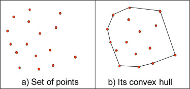
Fig.4: Example of a convex hull for a given point set

The Significance of the New Concavity Measure: The new concavity measure provides a more holistic understanding of the  concavity distribution throughout a 3D mesh. By identifying regions of concavity and analyzing the curvature around specific edges, this method offers valuable insights into the overall shape and structure of complex 3D geometries.

Our Understanding of the Convex Hull Algorithm: Before delving into the implementation of the new concavity measure, it is essential to  grasp the concept of the convex hull algorithm. 

The convex hull represents the smallest convex shape that encloses a set of points in 2D (a polygon) or 3D (a polyhedron). The widely used Quickhull algorithm follows steps such as finding extreme points, dividing and conquering, recursion, and merging to compute the convex hull efficiently.

What We Have Done: To calculate the new concavity measure for a given edge (v-w), the process involves the following steps:

a. Identifying touching triangles: Iterate through the mesh to find all triangles sharing the vertices v and w, defining the selected edge.

b. Creating a point set (P): Extract all vertices from the touching triangles and collect them into a single set, forming point set P. Each vertex represents a point in 3D space and contributes to the overall shape of the region around the selected edge. 

c. Computing the convex hull: Utilize the convex hull algorithm, such as the Quickhull algorithm, to determine the convex hull of point set P. The convex hull forms a closed shape that encloses all points in the point set.

d. Calculating the difference: Subtract the vertices of the convex hull from point set P to obtain the regions of concavity. These points represent areas where the mesh deviates inward and create indentations or concavities rather than forming part of the convex hull’s outer boundary.

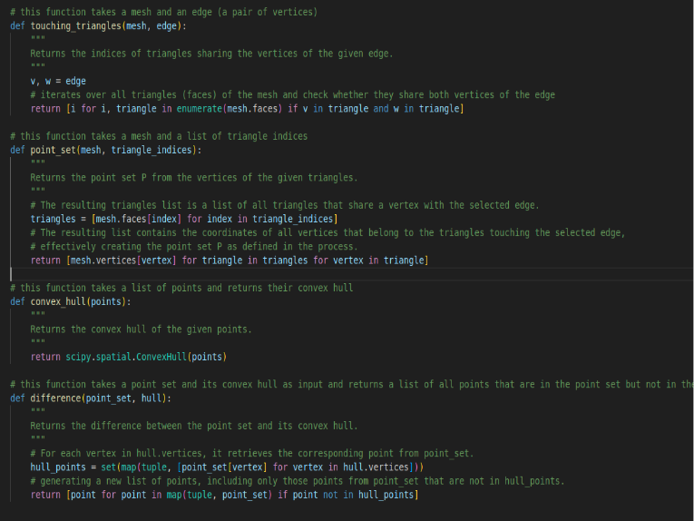
Fig.5: Our code block in python for the specified steps (a-d)

Repeating the Process for Other Edges: To explore concavity across different parts of the mesh, the entire process can be repeated for other edges. By selecting a new edge (v’-w’) and following the steps of creating a point set, computing the convex hull, and calculating the difference, we can gain unique insights into the concavity distribution and shape features across various regions of the 3D mesh.

Visualization and Interpretation: Visualizing the results of the new concavity measure allows for a more intuitive understanding of the regions exhibiting pronounced concavities. By analyzing the difference between the point set P and its convex hull, researchers and designers can identify critical areas with concavities, evaluate surface quality, and optimize the mesh shape if needed.

2.2 Insights into Mesh Decomposition

There are various algorithms and methods for performing 3D convex decomposition, and the complexity of these methods can vary depending on the input object’s complexity and the desired level of accuracy in the decomposition.

We worked on the idea based on the algorithm (Fig.6) by Approximate Convex Decomposition paper (Thul, D. et al. (2018) Approximate convex decomposition and transfer for animated meshes, ACM Transactions on Graphics. Available at: https://dl.acm.org/doi/10.1145/3272127.3275029.).  

Dividing the mesh through concave edges gives the exact solution but it is intractable; so as an approximation we decided to go with Breadth-First-Search (BFS) starting from each vertex. Then grow as long as no concave edge is visited. At the end, we tried to keep the maximum connected component guided by the two measures mentioned above.

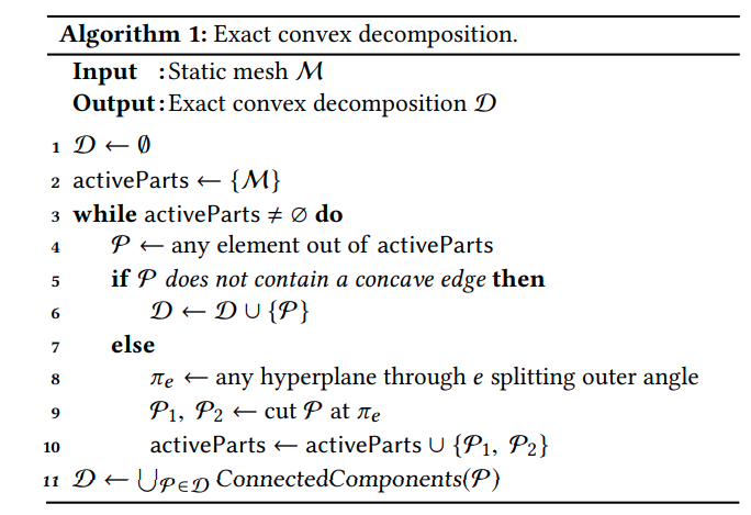
Fig.6: The exact mesh decomposition algorithm-Thul, D. et al. (2018)

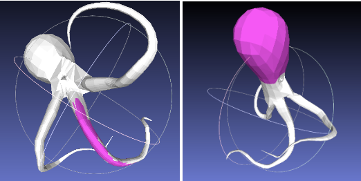
Fig.7: Highlighted regions identified as convex in 2.3. Visualized in MeshLab

2.3 An alternative approach:

A separate angle worked using a half-edge data structure to traverse the mesh. An existing half-edge data structure was heavily modified to suit the purposes of this project. The goal was to identify regions of faces connected only by convex edges using a breadth-first search, and then find the largest convex region. Early attempts resulted in non-planar regions, so the next iteration of the algorithm tracked the number of faces, edges and vertices and used the Euler formula for planar graphs to force the region of faces to remain a planar graph. 

The final iteration was to apply a rule that checked that new triangles were not outside the existing region (as determined by planes formed by triangles with a concave edge), while allowing for slightly concave edges, in addition to earlier rules. This process was similar to the process for exact 3D decomposition, except that the algorithm does not check whether existing triangles should be eliminated by new concave edges. Using this method resulted in slightly more reasonable shapes for the 5 largest “convex” regions on the squid (one such region is highlighted in the Fig. 7).

3. Conclusion:

Because of our time limit, we have looked at specific parts of decomposition techniques.

Here is our comparison for these two concavity measures: Computing dihedral angles is a simple and efficient method for detecting concave edges and can be combined with BFS search method to retrieve convex components.

On the other hand, the concavity measure using Qhull offers a powerful approach to analyzing 3D meshes and understanding concavity distribution in complex geometries. By identifying regions of concavity and analyzing curvature around specific edges, this method provides valuable insights for various applications in computer graphics, computational geometry, and engineering. The ability to repeat the process for different edges allows for a detailed exploration of concavity throughout the entire 3D mesh, leading to improved surface quality assessment and shape optimization. Embracing this new concavity measure will undoubtedly enhance our understanding of complex 3D geometries and contribute to advancements in computer graphics and design.