The (in)accurate Gradients of Neural Representations

Students: Gabriele Dominici, Daniel Perazzo, Munshi Sanowar Raihan, João Teixeira

TA: Nursena Koprucu

Mentors: Peter Yichen Chen, Rundi Wu, Honglin Chen, Ishit Mehta, Eitan Grinspun

1. Introduction

Implicit neural representation promises infinite resolution, automatic gradients, and memory efficiency. In practice, however, these promises often do not hold. Our project explored one specific drawback of implicit neural representations: the noisy gradient. The source code of this project is available on our GitHub repository.

The noisy gradient problem of neural representation has been observed in the context of solving PDEs [1], geometry processing [2,3], topology optimization [4], and 3D reconstruction [5].

1.1. Motivational Example: 1D advection

Our goal is to solve time-dependent PDEs on neural network-based spatial representations. Let’s consider the classic 1D advection equation:

This equation describes the passive advection of some scalar field u carried along at a constant speed a.

Fig 1: Advected scalar field (left), and gradient of the advected quantity (right) over time.

We will parameterize each time-discretized spatial field with a neural network. The field quantity at an arbitrary location can be queried via network inference f(x). The weights of this network are updated at each time step with optimization-based time integration [1]. 

1.2. The Problem: Noisy Gradients

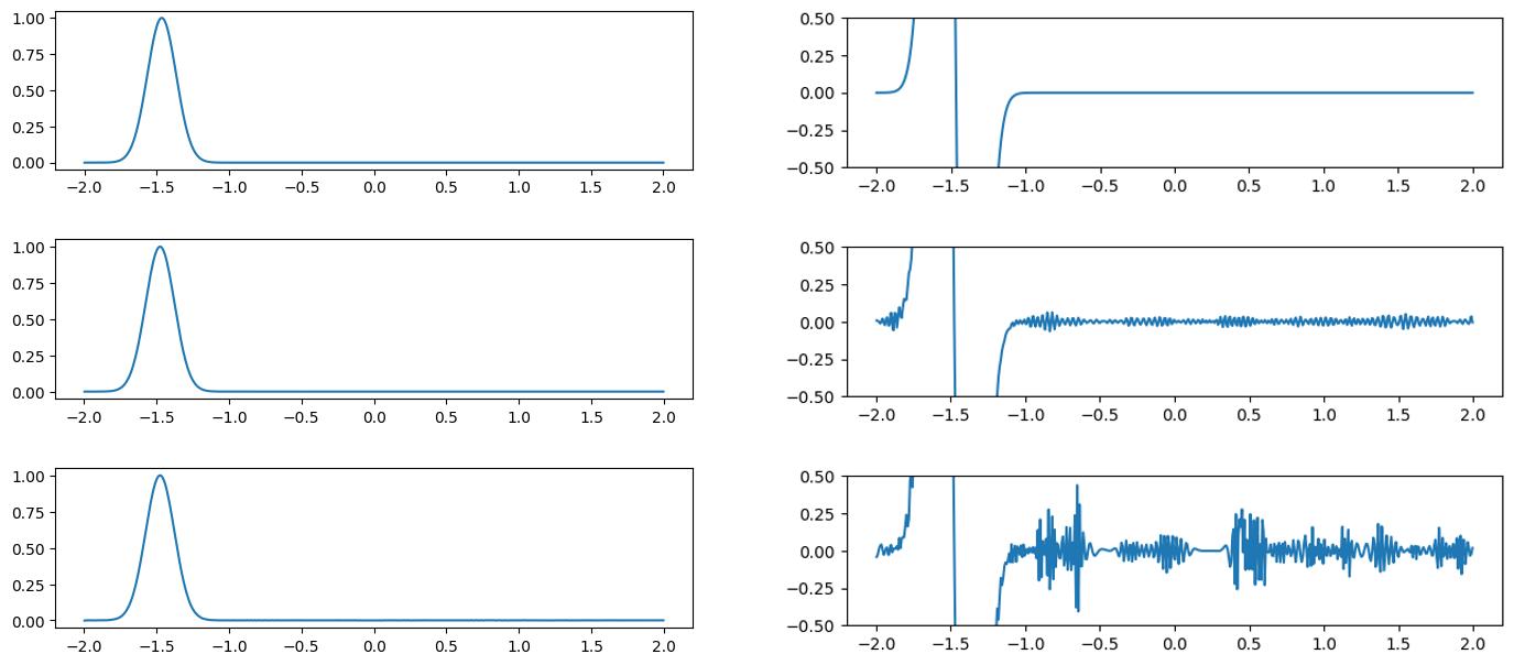
   Fig 2: Comparisons of advected values and gradients of different neural representations. Ground truth (top row), the sine activation (middle row), and the Gaussian activation (bottom row).

Following the INSR literature, we explore different activation functions for our neural network-based scalar field. The figure above compares the predicted scalar quantity and their gradients for both sine [8] and Gaussian [12] activation networks. The predicted scalar quantity matches the ground truth well in all cases. But the gradient of the advected quantity is extremely noisy regardless of the choice of the activation function.

In the subsequent sections, we will tackle this problem using several approaches that fall into two categories: pure neural representation (Section 2) and hybrid grid-neural representations (Section 3).

2. Pure Neural Representations

2.1 Tuning Omega

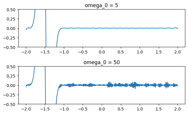
Fig 3: Large omega values cause noisy gradients, while small omega values give smoother gradients.

The omega hyperparameter controls the frequency range that the SIREN network learns [8]. In general, if we reduce the value of omega, the gradients learned by the networks become less noisy. As seen in the figure above, choosing omega = 5 ensures the network has smooth gradients, while choosing a larger value like 50 gives us very noisy gradients. However, finding the optimal omega value is a non-trivial task. Users need to tune this parameter for each problem.

2.2. Finite Differences

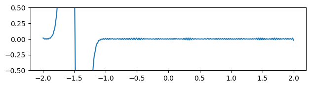
Fig 4: Gradients estimated by finite difference method.

Instead of calculating the gradients by taking the derivative of the output with respect to the inputs using autodiff, we can also use finite differences to approximate the gradients. Because finite difference stencils have local compact supports, they are less susceptible to noise. Indeed, the gradients of the finite difference solution are much less noisy than the autodiff version (see figure above).

2.3 Averaging

Fig 5: Evolving of the gradient of the function over time in the mean gradients approach.

Instead of using the gradients computed by autodiff, we spatially average them by calculating the mean at four more neighboring points for each location.  Although the gradients seem smoother at the very beginning, it is easy to see that after a few timesteps, the gradient’s peaks become fictitiously taller, degrading the results (Fig 5). 

2.4 Initializing with Ground Truth Gradients

Fig 6: Evolving of the gradient of the function over time where the gradients are initialized to be the ground truth gradients.

At timestep 0, the neural network is trained to predict the initial values of the function we are trying to optimize. In addition, similarly to what is done in Sobolev training [6], we force the model to have the same gradients as the desired function. 

This method does reduce the noise in the gradient over time (Fig 6), but the information gathered from the extra supervision used in the initialization steps slowly dissolves. Furthermore, these gradients are not always available or not suitable for setting up a loss function in such a manner, making this solution not always applicable. 

3. Hybrid grid-neural representations

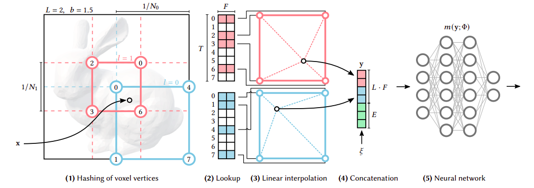
Fig 7: Description of the multi-resolution hashgrid (reproduced from [7]).

To address neural representations’ long training time, Muller et al. [7] developed a multi-resolution hash grid approach: instantNGP. In the following section, we explore instantNGP’s gradient quality. We benchmark it on a 2D fluid example. The figure below shows the example’s initial condition:

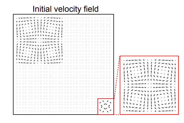
Fig 8: Vortex velocity field (reproduced from [1]).

When we try to fit this initial condition using a pure neural representation (i.e., NOT instantNGP), we observe highly noisy gradients, consistent with the results reported in Section 2.1.

Fig 9: Gradient we obtained using pure neural representations for the proposed 2D vortex problem.

Next, we investigated hybrid neural-grid representations, varying the type of the grids and the type of the hash (See Fig 10). 

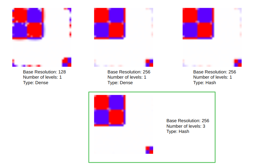
Fig 10: Different gradients for different resolutions.

The parameters outlined in green obtained the best result. In this case, we use a base resolution of 256 and a 3-level hash grid. 

However, those results only accounted for the initial conditions. If we let the gradients evolve for 99 timesteps according to the PDE, we observe that the gradients start diverging, as can be seen in the video below.

Fig 11: Evolution of the gradients for the 2D fluids for the two vortices example. This test was done with a dense grid of 512 resolution.

In summary, although our hybrid approach seems excellent for the first timesteps, it also appears to limit the expressivity of the network during subsequent evolution.

Due to these problems in the 2D Fluid scenario, we investigated the gradients’ performance in another environment: the 2D Advection problem.

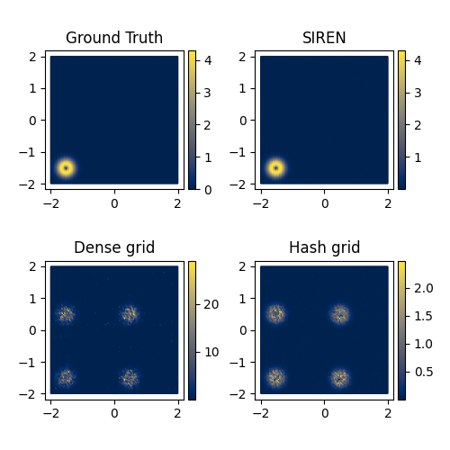
Fig 12: Comparison of Gradient Magnitudes for Different methods.

We used the same network configurations (base resolution, number of levels, number of hidden layers, and hidden features) as the 2D Fluid problem. The hybrid neural-grid representation performs significantly worse than the pure neural representation using SIREN (see Fig 12). Here the network is asked to fit the initial condition only.

Next, we tried to tune the configuration parameters. We discovered that the models performed better for the 2D Advection scenario when the number of level is increased. The best result is given by the following parameters:  number of Levels: 16; per Level Scale: 1.5; Base resolution: 16.

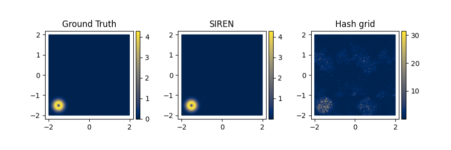
Fig 13: Comparison of Gradient Magnitudes for Hash grid’s best parameters.

Even though the hash grid’s performances improved, the figure above demonstrates that the gradients are still much noisier than the pure neural representation (SIREN). 

As such, we conclude that the hybrid grid-neural representation’ performance is not consistently better than the pure neural representation. In fact, it’s sometimes worse, as demonstrated in the 2D advection example.

4. Future Work

Since our tests and other SIREN works [8] show that tuning the omega hyperparameter is essential for the gradient results, one possible next step is to perform automatic gradient tuning, as proposed in meta-learning techniques [9].

Another possible approach is supervising the gradients. Instead of using the original function to compute the gradients, it is possible to use a separate loss function that certifies the correct gradient values over time. Essentially, we aim to write down the evolution equation of the gradient itself and couple this equation with the original PDE.

Future work should also consider a theoretical understanding of the gradient problem. One possible cause for this problem is the global non-compact support of neural networks. This initially motivates us to explore hybrid grid-neural networks. Other works [7, 10, 11] used similar approaches to extract local features to feed into the network, enforcing a locality to the neural network.

5. References

[1] Chen, Honglin, Wu Rundi, Eitan Grinspun, Changxi Zheng, and Peter Yichen Chen. “Implicit Neural Spatial Representations for Time-dependent PDEs.” International Conference on Machine Learning (ICML). 2023.

[2] Mehta, Ishit, Manmohan Chandraker, and Ravi Ramamoorthi.” A level set theory for neural implicit evolution under explicit flows.” European Conference on Computer Vision (ECCV).  2022.

[3] Yang, Guandao, Serge Belongie, Bharath Hariharan, and Vladlen Koltun. “Geometry processing with neural fields.” Neural Information Processing Systems (NeurIPS). 2021.

[4] Zehnder, Jonas, Yue Li, Stelian Coros, and Bernhard Thomaszewski. “Ntopo: Mesh-free topology optimization using implicit neural representations.” Neural Information Processing Systems (NeurIPS). 2021.

[5] Verbin, Dor, Peter Hedman, Ben Mildenhall, Todd Zickler, Jonathan T. Barron, and Pratul P. Srinivasan. “Ref-nerf: Structured view-dependent appearance for neural radiance fields.” Conference on Computer Vision and Pattern Recognition (CVPR).  2022.

[6] Czarnecki, Wojciech M., Simon Osindero, Max Jaderberg, Grzegorz Swirszcz, and Razvan Pascanu. “Sobolev training for neural networks.” Neural Information Processing Systems (NeurIPS). 2017.

[7] Müller, Thomas, Alex Evans, Christoph Schied, and Alexander Keller. “Instant neural graphics primitives with a multiresolution hash encoding.” ACM Transactions on Graphics (ToG) 41. 2022.

[8] Sitzmann, Vincent, Julien Martel, Alexander Bergman, David Lindell, and Gordon Wetzstein. “Implicit neural representations with periodic activation functions.” Neural Information Processing Systems (NeurIPS). 2020.

[9] Hospedales, Timothy, Antreas Antoniou, Paul Micaelli, and Amos Storkey. “Meta-learning in neural networks: A survey.” IEEE transactions on pattern analysis and machine intelligence 44.9. 2021.

[10] Sun, Cheng, Min Sun, and Hwann-Tzong Chen. “Direct voxel grid optimization: Super-fast convergence for radiance fields reconstruction.” Conference on Computer Vision and Pattern Recognition (CVPR). 2022.

[11] Barron, Jonathan T., Ben Mildenhall, Dor Verbin, Pratul P. Srinivasan, and Peter Hedman. “Zip-NeRF: Anti-aliased grid-based neural radiance fields.”  International Conference on Computer Vision (ICCV). 2023.

[12] Shin-Fang Chng, Sameera Ramasinghe, Jamie Sherrah, Simon Lucey. “Gaussian Activated Radiance Fields for High Fidelity Reconstruction and Pose Estimation” The European Conference on Computer Vision (ECCV). 2022.