By SGI Fellows: Anna Cole, Francisco Unai Caja López, Matheus da Silva Araujo, Hossam Mohamed Saeed
Mentor: Paul Kry
Volunteers: Leticia Mattos Da Silva and Erik Amézquita
I. Introduction
This technical report describes a follow-up to our previous post. One of the original goals of the project was to apply successive self-parameterization to solve differential equations on curved surfaces leveraging a multigrid solver based on Liu et al. 2021. This post reports the results obtained throughout the summer to achieve this objective and wraps-up the project. Video 1 shows an animation of heat diffusion, obtained by solving the heat equation on surface meshes using the geometric multigrid solver.
II. Partial Differential Equations
Partial differential equations (PDEs) are equations that relate multiple independent variables and their partial derivatives. In graphics and animation applications, PDEs usually involve time derivatives and spatial derivatives, e.g., the motion of an object in 3D space through time described by a function \(f(x, y, z, t)\). Frequently, a set of relationships between partial derivatives of a function is given and the goal is to find functions \(f\) satisfying these relationships.
To more easily study and analyze these equations, it is possible to classify them according to the physical phenomena they describe, which are briefly summarized below. Solomon 2015 and Heath 2018 provide extensive details on partial differential equations for those interested in more in-depth discussions on the topic.
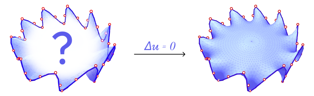
Elliptic PDEs are PDEs that describe systems that have already reached an equilibrium (or steady) state. One example of elliptic PDE is the Laplace equation, given by \(\bigtriangleup \mathbf{u} = \mathbf{0}\). Intuitively, starting with values known only at the boundary of the domain (i.e., the boundary conditions), this equation finds a function \(\mathbf{u}\) such that the values in the interior of the domain smoothly interpolate the boundary values. Figure 1 illustrates this description.
Parabolic PDEs are equations that describe systems that are evolving towards an equilibrium state, usually related to dissipative physical behaviour. The canonical example of a parabolic PDE is the heat equation, defined as \(\frac{\mathrm{d}}{\mathrm{dt}} \mathbf{u} = \bigtriangleup \mathbf{u}\). The function \(\mathbf{u}\) describes how heat flows with time over the domain, given an initial heat distribution that describes the boundary conditions. This behaviour can be visualized in Animation 1.
Finally, hyperbolic PDEs describe conservative systems that are not evolving towards an equilibrium state. The wave equation, described by \(\frac{\mathrm{d}^2}{\mathrm{dt^{2}}} \mathbf{u} = \bigtriangleup \mathbf{u}\), is the typical example of a hyperbolic PDE. In this case, the function \(\mathbf{u}\) characterizes the motion of waves across elastic materials or the motion of waves across the surface of water. Animation 2 provides a visual illustration of this phenomenon. One striking difference between the wave equation and the heat equation is that for the former it is not enough to specify initial conditions for \(\mathbf{u}\) at time \(t = 0\); it is also necessary to define initial conditions for the derivatives \(\mathbf{\frac{\mathrm{d}}{\mathbf{dt}} \mathbf{u}}\) at time \(t = 0\).
In this project, we restricted the implementation to solving the heat diffusion equations on curved triangle meshes (see Crane et al. 2013). This leads to the following time discretization using a backward Euler step:
\(\begin{equation} \frac{\mathrm{d}}{\mathrm{dt}} \mathbf{u} = \bigtriangleup \mathbf{u} \rightarrow (\mathbf{I} – t\mathbf{L}) \mathbf{u}_{t} = \mathbf{u}_{0} \end{equation}\)
where \(\mathbf{u}_{0}\) is the initial heat distribution and \(\mathbf{L}\) is the Laplacian.
To spatially discretize the equation, we used the cotan-Laplacian \(\mathbf{L}\) discretized at a vertex \(i\):
\(\begin{equation} (\mathbf{L}u){i} = \frac{1}{2 A_{i}} \sum_{j \in \mathcal{N}_{i}} \left(\cot \alpha_{ij} + \cot \beta_{ij} \right) \left(u_{j} – u_{i} \right) \end{equation}\)
where \(A_{i}\) is one-third of the sum of the areas of all the triangles incident to vertex \(i\), \(\mathcal{N}_{i}\) denotes the set of adjacent vertices, and \(\alpha_{ij}, \beta_{ij}\) are the angles that oppose the edge \(e_{ij}\) connecting vertex \(i\) to its neighbor \(j\). The result is a linear system \(\mathbf{A}\mathbf{x} = \mathbf{b}\), where \(\mathbf{A} = \mathbf{I} – t\mathbf{L}\) and \(\mathbf{b} = \mathbf{u}_{0}\). This linear system can be solved numerically.
III. Multigrid Method
There is a large variety of methods to numerically solve PDEs. After choosing time and spatial discretization, the PDE may be solved as a linear system. To that end, it is possible to apply a direct solver (e.g., LU decomposition or Cholesky factorization) to find the solution. These methods are exact in the sense that they provide an exact solution in a finite number of steps. One disadvantage of direct solvers approach is that it may be too expensive to frequently recompute the matrix decomposition in cases where the system of equations requires updates. Iterative methods (e.g., Gauss-Seidel and Jacobi) provide an efficient alternative, but at the cost of providing only approximate solutions and having poor rates of convergence. Multigrid methods attempt to improve the convergence of iterative solvers by creating a hierarchy of meshes and solving the linear system in a hierarchical manner.
Iterative methods usually rapidly remove high-frequency errors, but slowly reduce low-frequency errors. This significantly affects the rate of convergence. The key observation of multigrid solvers is that low-frequency errors on the domain where the solution is defined (i.e., a grid or mesh) correspond to high-frequency errors on a \emph{coarser} domain. Hence, by simplifying the domain of the solution and transferring the errors from the original domain to a simplified one, an iterative solver can be used again on the coarse domain. The final result is that both high-frequency and low-frequency errors will be reduced in the original domain. See Solomon 2015 and Heath 2018 for details on numerical solutions for partial differential equations, and Botsch et al. 2010 for a discussion of multigrid methods applied to geometry processing in particular.
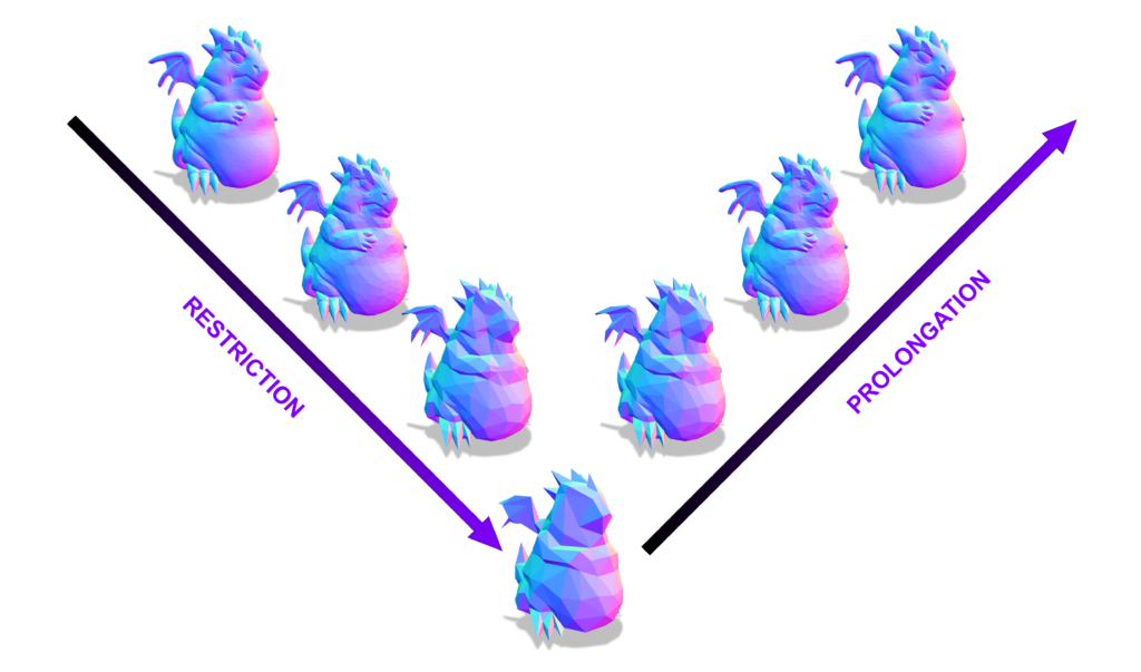
To transfer residuals from a fine level to a coarse level, a restriction operator must be defined, while the transfer from a coarse level to a fine level requires a prolongation operator that interpolates the solution found on coarse meshes to fine ones. This concept is illustrated in Figure 2 through a cycle of restriction and prolongation operators applied to a hierarchy of meshes. The method requires both a hierarchy of grids or meshes and a suitable mapping between successive levels of the hierarchy. For structured domains, such as grids, restriction and prolongation operators are well-established due to the regularity of the domain (Brandt 1977). For unstructured domains, such as curved surface meshes, it is harder to define a mapping between different levels of the hierarchy. To this end, Liu et al. 2021 proposes an intrinsic prolongation operator based on the successive self-parameterization of Liu et al. 2020, discussed in our previous report. To summarize, successive self-parameterization creates a bijective mapping between successive levels of the hierarchy, making it feasible to transfer back-and-forth the residuals in both directions (fine-to-coarse and coarse-to-fine). To achieve this, quadric mesh simplification is used to create the hierarchy of meshes and conformal parameterization is employed to uniquely correspond points on successive hierarchical levels.
Using the intrinsic prolongation operator matrix \(\mathbf{P}_{h}\) and the restriction operator matrix \(\mathbf{R} = \mathbf{P}_{h}^{T}\) for a level \(h\) of the hierarchy, where each level of the hierarchy has different prolongation/restriction matrices, the multigrid algorithm can be summarized as follows (Liu et al. 2021, Heath 2018):
- Inputs: a system matrix \(\mathbf{A}\), the right-hand side of the linear system \(\mathbf{b}\), and a sequence of prolongation-restriction operators for the hierarchy.
- Pre-Smoothing: at level \(h\) of the hierarchy, compute an approximate solution \(\hat{\mathbf{x}}\) for the linear system \(\mathbf{A} \mathbf{x} = \mathbf{b}\) using a smoother (for instance, the Gauss-Seidel solver). A small number of iterations should be used in the smoothing process.
- Compute the residual and transfer it to the next level of the hierarchy (a coarse mesh): \(\mathbf{r} = \mathbf{P}_{h + 1}^{T} \left(\mathbf{b} – \mathbf{A} \hat{\mathbf{x}} \right)\). The system matrix of the next level is given by \(\mathbf{\hat{A}} = \mathbf{P}_{h+1}^{T}\mathbf{A}\mathbf{P}_{h+1}\).
- Recursively apply the method using the residual found in the previous step and return the solution \(\mathbf{c}_{h+1}\) found in the next level of the hierarchy. As the base case, a direct solver can be used at the coarsest level of the hierarchy. This should be efficient, since the system to be solved will be small at the coarsest level.
- Interpolate the results found by the method at the next level of the hierarchy using the prolongation operator: \(\mathbf{x}’ = \mathbf{P}_{h + 1} \mathbf{c}_{h+1}\).
- Post-Smoothing: apply a small number of iterations of a smoother (e.g., the Gauss-Seidel solver) on the solution found in the previous step.
For the sake of completeness, the multigrid solver described is more specifically an example of a geometric multigrid method, since the system was simplified using the geometry of the mesh or domain. In contrast, an algebraic multigrid method constructs a hierarchy from the system matrix without additional geometric information. Moreover, the hierarchy traversal described (going from finest to coarsest and back to finest) is known as a V-cycle multigrid, but there are many possible variants such as W-cycle multigrid, full multigrid and cascading multigrid. Again, we refer the reader to Heath 2018 and Botsch et al. 2010 for details.
IV. Experiments and Results
Figure 3 through Figure 7 show a comparison of the geometric multigrid solver against a standard Gauss-Seidel solver with respect to the number of iterations for various surface meshes. The iterative process stopped when either the residual was below a certain threshold or after a number of iterations. For all the experiments, the threshold used was \(\epsilon = 10^{-11}\) and the maximum number of iterations was \(3000\). For the geometric multigrid solver, the plots show the total number of smoothing iterations, and not the total number of V-Cycles. In all experiments, \(5\) pre-smoothing and \(5\) post-smoothing iterations were used for the geometric multigrid solver.
As can be seen in the plots of Figure 3 to Figure 7, the Gauss-Seidel stopped due to the maximum iterations criteria for all but one experiment (Figure 3, Spot (Low Poly)). For all the others, the solution found is above the specified threshold. In contrast, the geometric multigrid solver quickly converges to a solution below the desired threshold.
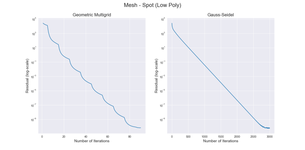
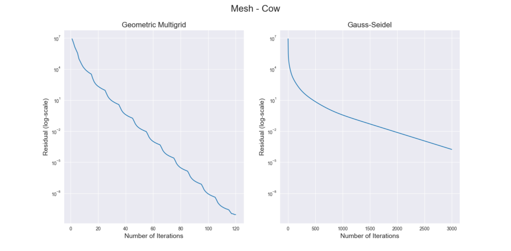
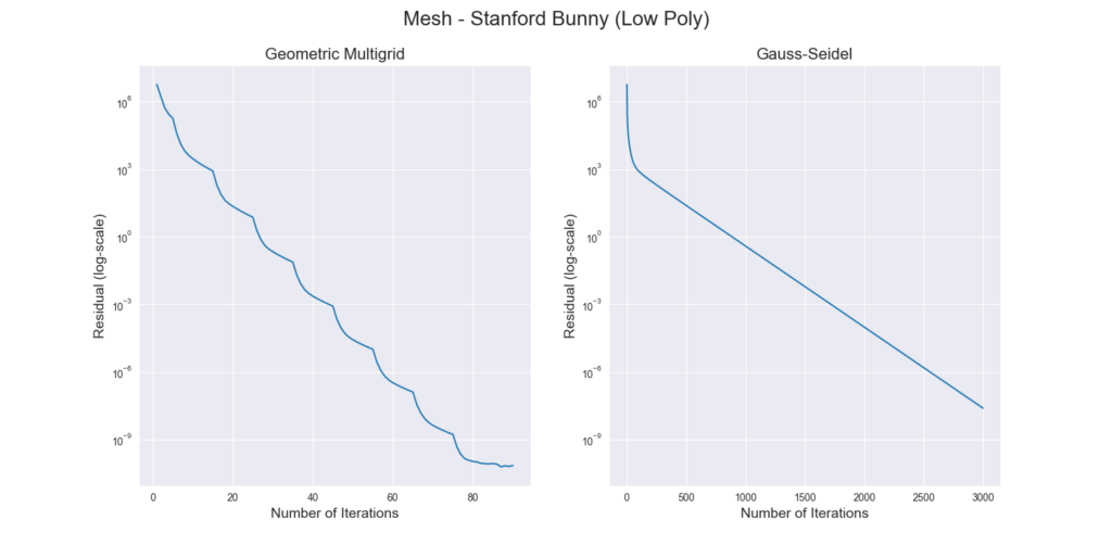
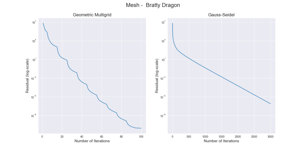

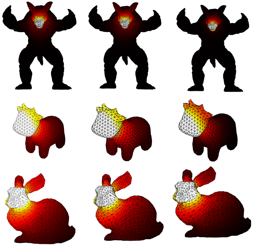
Figure 8 presents a visual comparison of a ground-truth solution (Figure 8, left) and the solutions found by the geometric multigrid solver (Figure 8, center) and the Gauss-Seidel solver (Figure 8, right). The geometric multigrid matches more closely the expected solution, while the solution computed by the Gauss-Seidel solver fails to correctly spread the heat distribution.
Finally, Figure 9 and Figure 10 compare the execution time of the geometric multigrid solver against the Gauss-Seidel solver. However, the multigrid method requires the construction of a hierarchy of meshes through the mesh simplification algorithm, which is not required for the Gauss-Seidel method. As the results demonstrate, the geometric multigrid version is faster than the Gauss-Seidel method even when the time to compute the successive self-parameterization is taken into account.
One limitation of our MATLAB implementation is that the system runs out of memory for some of the input meshes. To run all the experiments with the same parameters, we limited the hierarchy depth to two, which would correspond to a two-grid algorithm. However, Heath 2018 mentions that deeper hierarchies can make the computation progressively faster. Hence, we could expect even better results using an optimized implementation.


V. Conclusions and Future Work
In this post we report the results obtained for the geometric multigrid solver for curved meshes, which was one of the original goals of the SGI project proposal. With this, the SGI project can be considered complete. The implementation may be improved in various aspects, especially regarding memory usage, which was a critical bottleneck in our case. For this, an implementation in a low-level language that provides fine-grained control over memory allocation and deallocation may be fruitful. Moreover, a comparison with Wiersma et al. 2023 could be an interesting direction for further studies in the area and to investigate new research ideas.
We would like to profusely thank Paul Kry for the mentoring, including the patience to keep answering questions after the two weeks scheduled for the project.
VI. References
Liu, H., Zhang, J., Ben-Chen, M. & Jacobson, A. Surface Multigrid via Intrinsic Prolongation. ACM Trans. Graph. 40 (2021).
Solomon, Justin. Numerical algorithms: methods for computer vision, machine learning, and graphics. CRC press, 2015.
Heath, Michael T. Scientific computing: an introductory survey, revised second edition. Society for Industrial and Applied Mathematics, 2018.
Crane, Keenan, Clarisse Weischedel, and Max Wardetzky. “Geodesics in heat: A new approach to computing distance based on heat flow.” ACM Transactions on Graphics (TOG) 32.5 (2013): 1-11.
Botsch, Mario, et al. Polygon mesh processing. CRC press, 2010.
Brandt, Achi. “Multi-level adaptive solutions to boundary-value problems.” Mathematics of computation 31.138 (1977): 333-390.
Liu, H., Kim, V., Chaudhuri, S., Aigerman, N. \& Jacobson, A. Neural Subdivision. ACM Trans. Graph.. 39 (2020).
Wiersma, Ruben, et al. “A Fast Geometric Multigrid Method for Curved Surfaces.” ACM SIGGRAPH 2023 Conference Proceedings. 2023.