Categories
Research

3D Reconstruction of the Underwater Sea-floor

Students: Daniel Perazzo, Sanowar Munshi, Francheska Kovacevic

TA: Kevin Roice

Mentors: Antonio Teran, Zachary Randell, Megan Williams

Introduction

Monitoring the health and sustainability of native ecosystems is an especially pressing issue in an era heavily impacted by global warming and climate change. One of the most vulnerable types of ecosystems for climate change are the oceans, which means that developing methods to monitor these ecosystems is of paramount importance. 

Inspired by this problem, this SGI 2023 project aims to use state-of-the-art 3D reconstruction methods to monitor kelp, a type of algae that grows in Seattle’s bay area.

This project was done in partnership with Seattle aquarium and allowed us to use data available from their underwater robots as shown in the figure below.

Figure 1: Underwater robot to collect the data

This robot collected numerous pictures and videos in high-resolution, as seen in the figure below. From this data, we managed to perform the reconstruction of the sea floor, by some steps. First we perform a sparse reconstruction to get the camera poses and then we perform some experiments to perform the dense reconstruction. The input data is shown below.

Figure 2: Types of input data extracted by the robot. High-resolution images for 3D reconstruction

Sparse Reconstruction

To get the dense reconstruction working, we first performed a sparse reconstruction of the scene, in the image below we see the camera poses extracted using COLMAP [5], and their trajectory in the underwater seafloor. It should be noted that the trajectory of the camera differs substantially from the trajectory of the real robot. This could be caused by the lack of a loop closure during the trajectory of the camera. 

Figure 3: Camera poses extracted from COLMAP. 

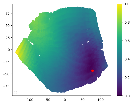
With these camera poses, we can reconstruct the depth maps, as shown below. These are very good for debugging, since we can visualize and get a grasp of how the output of COLMAP differs from the real result. As can be seen, there are some artifacts for the reconstruction of the depth for this image. And this will reflect in the quality of the 3D reconstruction.

Figure 4: Example of depth reconstruction using the captured camera poses extracted by COLMAP

3D Reconstruction

After computing the camera poses, we can go to the 3D reconstruction step. We used some techniques to perform 3D reconstruction of the seafloor using the data provided to us by Dr. Zachary Randell and his team. For our reconstruction tests we used COLMAP [1]. In the image below we present the image of the reconstruction.

Figure 5: Reconstruction of the sea-floor.

We can notice that the reconstruction of the seabed has a curved shape, which is not reflected in the real seabed. This error could be caused by the fact that, as mentioned before, this shape has a lack of a loop closure.

We also compared the original images, as can be seen in the figure below. Although “rocky”, it can be seen that the quality of the images is relatively good.

Figure 6: Comparison of image from the robot video with the generated mesh.

We also tested with NeRFs [2] in this scene using the camera poses extracted by COLMAP. For these tests, we used nerfstudio [3]. Due to the problems already mentioned for the camera poses, the results of the NeRF reconstruction are really poor, since it could not reconstruct the seabed. The “cloud” error was supposed to be the reconstructed view. An image for this result is shown below:

Figure 7: Reconstruction of our scene with NeRFs. We hypothesize this being to the camera poses.

We also tested with a scene from the Sea-thru-NeRF [4] dataset, which yielded much better results:

Figure 8: Reconstruction of Sea-thru-NeRF with NeRFs. The scene was already prepared for NeRF reconstruction

Although the perceptual results were good, for some views, when we tried to recover the results using NeRFs yielded poor results, as can be seen on the point cloud bellow:

Figure 9: Mesh obtained from Sea-thru-NeRF scene. 

As can be seen, the NeRF interpreted the water as an object. So, it reconstructed the seafloor wrongly.

Conclusions and Future Work

3D reconstruction of the underwater sea floor is really important for monitoring kelp forests. However, for our study cases, there is a lot to learn and research. More experiments could be made that perform loop closure to see if this could yield better camera poses, which in turn would result in a better 3D dense reconstruction. A source for future work could be to prepare and work in ways to integrate the techniques already introduced on Sea-ThruNeRF to nerfstudio, which would be really great for visualization of their results. Also, the poor quality of the 3D mesh generated by nerfstudio will probably increase if we use Sea-ThruNeRF. These types of improvements could yield better 3D reconstructions and, in turn, better monitoring for oceanographers.

References

[1] Schonberger, Johannes et al. “Structure-from-motion revisited.” IEEE Conference on Computer Vision and Pattern Recognition (CVPR). 2016.

[2] Mildenhall, Ben, et al. “Nerf: Representing scenes as neural radiance fields for view synthesis.” Communications of the ACM. 2021

[3] Tancik, M., et al. “Nerfstudio: A modular framework for neural radiance field development”. ACM SIGGRAPH 2023.

[4] Levy, D., et al. “SeaThru-NeRF: Neural Radiance Fields in Scattering Media.” IEEE/CVF Conference on Computer Vision and Pattern Recognition (CVPR). 2023.

[5] Schonberger, Johannes L., and Jan-Michael Frahm. “Structure-from-motion revisited.” IEEE/CVF Conference on Computer Vision and Pattern Recognition (CVPR). 2016.

Categories
Research

A Study on Quasimetric Reinforcement Learning

Students: Gabriele Dominici, Daniel Perazzo, Munshi Sanowar Raihan, Biruk Abere, Sana Arastehfar

TA: Jiri Mirnacik

Mentor: Tongzhou Wang

Introduction

In reinforcement learning (RL), an agent is placed in an environment, and is required to complete some task from a starting state. Traditionally, RL is often studied under the single-task setting, where the agent is taught to do one task and one task only. However, multi-task agents are much more general and useful. A robot that knows to do all household tasks is much more valuable than one that only opens the door. In particular, many useful tasks of interest are goal-reaching tasks, i.e., reaching a specific given goal state from any starting state. 

Each RL environment implicitly defines a distance-like geometry on its states: 

“distance”(state A, state B) := #steps needed for an agent to go from state A to state B.

Such a distance-like object is called a quasimetric. It is a relaxation of the metric/distance function in that it can be asymmetrical (i.e., d(x,y) != d(y,x) in general). For example, 

  1. Going up a hill is harder than going down the hill. 
  2. Dynamic systems that model velocity are generally asymmetrical (irreversible).


Asymmetrical & irreversible dynamics occur frequently in games, e.g., this ice-sliding puzzle.
(Game: Professor Layton and Pandora’s Diabolical Box)

This quasimetric function captures how the environment evolves with respect to agent behavior. In fact, for any environment, its quasimetric is exactly what is needed to efficiently solve all goal-reaching tasks.  

Quasimetric RL (QRL)  is a goal-reaching RL method via learning this quasimetric function. By training on local transitions (state, action, next state), QRL learns to embed states into a latent representation space, where the latent quasimetric distance coincides with the quasimetric geometry for the environment. See https://www.tongzhouwang.info/quasimetric_rl/ for details.

The QRL paper explores the control capabilities of the learned quasimetric function, but not the representation learning aspects. In this project, we aim to probe the properties of learned latent spaces, which have a quasimetric geometry that is trained to model the environment geometry. 

Setup. We design grid-world-like environments, and use an provided implementation of QRL in PyTorch to train QRL quasimetric functions. Afterwards, we perform qualitative and visual analyses on the learned latent space.

Environments

Gridworld with directions

In reinforcement learning for the Markov decision process,  the agent has access to the internal state of the world. When the agent takes an action, the environment changes accordingly and returns the new state. In our case, we try to simulate a robot trying to reach a goal.

Our agent has only three actions: go forward, turn right and turn left. We assume that the agent has reached the goal if it is around the goal with a small margin of error. For simplicity, we fix the initial position and the goal position. We set the angular velocity and the step size to be fixed for the robot.

The environment returns to the agent the position it is currently in, and the vector direction the robot is currently facing. Following the example in the original QRL paper, we have a constant reward of -1 for the agent which encourages the agent to reach the goal as quickly as possible.

Training

For this project, we tested QRL on the aforementioned environments, where we obtained some interesting results. Firstly, we performed an offline version of QRL using only a critic network. For this setting, we used a dataset of trajectories created by actors performing a random trajectory. This random trajectory is then loaded when training starts.As shown in the figure in the previous section, we have a robot performing a random trajectory.

We trained in QRL varying the parameters for training the neural network. Using QRL we let the network train for various steps, as can be seen below:

After performing this training we analysed what would the agent learn, however, unfortunately, it seems that the agent is stuck, as can be seen in the figure below:

To get a better understanding of the problem, we performed some experiments using A2C implementation from stable_baselines. Instead of using the angle set-up as mentioned early, we used a setting where we return the angle directly. We also performed various runs, ~10 for A2C and always testing the trajectories. Although there were some runs that A2C did not manage to find the right trajectory, on some it did. We show the best results bellow:

We also performed some tests varying the parameters for quasimetric learning and inserting an intermediary state for the agent to reach the goal. After varying some parameters, including batch size and the coordinate space the agent is traversing. The improved results can be seen bellow, where the agents manage to reach the goal. Also, instead of, during the visualization, instead of using a greedy approach we instead use a categorical distribution, varying a temperature parameter to make it more random: 

These results were preliminary and we will not analyze these results for the next section.

We also performed an analysis on different settings, using different weights for our dynamic loss and and varying the previously mentioned temperature parameter. The table is shown bellow

Analyses

As previously said, we inspect the latent space learnt by the neural network to represent each state. In such a manner, it would be possible to inspect how the model reasons about the environment and the task. 

To do so, we sampled via a grid of parameters the state space of the Gridworld with directions environment. The grid was computed across 50 x values, 50 y values and 16 angle values equally separated. Then, we stored the latent representation computed by the model for each state and applied a t-SNE dimensionality reduction to qualitative evaluate the latent space referred to the state space. 

Figure 6: t-SNE representation of the latent space of the state space. The color represents the normalized predicted quasimetric distance between that state and the goal (red dot).

Figure 6 shows how these latent spaces learned by the model are meaningful with respect to the predicted quasimetric distance between two states. Inspecting it more in depth, it is possible to see how it also has some properties in this environment. Mostly, if you move along the x-axis in the reduced space, you advance in the y-axis in the env with different angles, while if you move along the y-axis in the reduced space, you advance in the x-axis in the environment. In addition, we believe that this behavior would also be present in other environments, but it needs further analysis. 

We also inspect the latent space learnt at different levels of the network (e.g. after including the possible actions and after the encoder in the quasimetric network), and all of them have similar representations. 

Conclusion & Future directions

Even in basic environments with limited action spaces, understanding the decision-making of agents with policies learned by neural networks can be challenging. Visualization and analysis of the learned latent space provide useful insights, but they require careful interpretation as results can be misleading.

As quasimetric learning is a nuanced topic, many problems from this week remain open and there are several interesting directions to pursue after these initial experiments:

  • Investigate the performance of quasimetric learning in various environments. What general properties of the environment are favorable for this approach?
  • Analyze world-models and multi-step planning. In this project, we examined only a 1-step greedy strategy.
  • Formulate and analyze quasimetric learning within a multi-environment context.
  • Design and evaluate more intricate environments suitable for real robot control
Categories
Research

The (in)accurate Gradients of Neural Representations

Students: Gabriele Dominici, Daniel Perazzo, Munshi Sanowar Raihan, João Teixeira

TA: Nursena Koprucu

Mentors: Peter Yichen Chen, Rundi Wu, Honglin Chen, Ishit Mehta, Eitan Grinspun

1. Introduction

Implicit neural representation promises infinite resolution, automatic gradients, and memory efficiency. In practice, however, these promises often do not hold. Our project explored one specific drawback of implicit neural representations: the noisy gradient. The source code of this project is available on our GitHub repository.

The noisy gradient problem of neural representation has been observed in the context of solving PDEs [1], geometry processing [2,3], topology optimization [4], and 3D reconstruction [5].

1.1. Motivational Example: 1D advection

Our goal is to solve time-dependent PDEs on neural network-based spatial representations. Let’s consider the classic 1D advection equation:

This equation describes the passive advection of some scalar field u carried along at a constant speed a.

Fig 1: Advected scalar field (left), and gradient of the advected quantity (right) over time.

We will parameterize each time-discretized spatial field with a neural network. The field quantity at an arbitrary location can be queried via network inference f(x). The weights of this network are updated at each time step with optimization-based time integration [1]. 

1.2. The Problem: Noisy Gradients

   Fig 2: Comparisons of advected values and gradients of different neural representations. Ground truth (top row), the sine activation (middle row), and the Gaussian activation (bottom row).

Following the INSR literature, we explore different activation functions for our neural network-based scalar field. The figure above compares the predicted scalar quantity and their gradients for both sine [8] and Gaussian [12] activation networks. The predicted scalar quantity matches the ground truth well in all cases. But the gradient of the advected quantity is extremely noisy regardless of the choice of the activation function.

In the subsequent sections, we will tackle this problem using several approaches that fall into two categories: pure neural representation (Section 2) and hybrid grid-neural representations (Section 3).

2. Pure Neural Representations

2.1 Tuning Omega

Fig 3: Large omega values cause noisy gradients, while small omega values give smoother gradients.

The omega hyperparameter controls the frequency range that the SIREN network learns [8]. In general, if we reduce the value of omega, the gradients learned by the networks become less noisy. As seen in the figure above, choosing omega = 5 ensures the network has smooth gradients, while choosing a larger value like 50 gives us very noisy gradients. However, finding the optimal omega value is a non-trivial task. Users need to tune this parameter for each problem.

2.2. Finite Differences

Fig 4: Gradients estimated by finite difference method.

Instead of calculating the gradients by taking the derivative of the output with respect to the inputs using autodiff, we can also use finite differences to approximate the gradients. Because finite difference stencils have local compact supports, they are less susceptible to noise. Indeed, the gradients of the finite difference solution are much less noisy than the autodiff version (see figure above).

2.3 Averaging

Fig 5: Evolving of the gradient of the function over time in the mean gradients approach.

Instead of using the gradients computed by autodiff, we spatially average them by calculating the mean at four more neighboring points for each location.  Although the gradients seem smoother at the very beginning, it is easy to see that after a few timesteps, the gradient’s peaks become fictitiously taller, degrading the results (Fig 5). 

2.4 Initializing with Ground Truth Gradients

Fig 6: Evolving of the gradient of the function over time where the gradients are initialized to be the ground truth gradients.

At timestep 0, the neural network is trained to predict the initial values of the function we are trying to optimize. In addition, similarly to what is done in Sobolev training [6], we force the model to have the same gradients as the desired function. 

This method does reduce the noise in the gradient over time (Fig 6), but the information gathered from the extra supervision used in the initialization steps slowly dissolves. Furthermore, these gradients are not always available or not suitable for setting up a loss function in such a manner, making this solution not always applicable. 

3. Hybrid grid-neural representations

Fig 7: Description of the multi-resolution hashgrid (reproduced from [7]).

To address neural representations’ long training time, Muller et al. [7] developed a multi-resolution hash grid approach: instantNGP. In the following section, we explore instantNGP’s gradient quality. We benchmark it on a 2D fluid example. The figure below shows the example’s initial condition:

Fig 8: Vortex velocity field (reproduced from [1]).

When we try to fit this initial condition using a pure neural representation (i.e., NOT instantNGP), we observe highly noisy gradients, consistent with the results reported in Section 2.1.

Fig 9: Gradient we obtained using pure neural representations for the proposed 2D vortex problem.

Next, we investigated hybrid neural-grid representations, varying the type of the grids and the type of the hash (See Fig 10). 

Fig 10: Different gradients for different resolutions.

The parameters outlined in green obtained the best result. In this case, we use a base resolution of 256 and a 3-level hash grid. 

However, those results only accounted for the initial conditions. If we let the gradients evolve for 99 timesteps according to the PDE, we observe that the gradients start diverging, as can be seen in the video below.

Fig 11: Evolution of the gradients for the 2D fluids for the two vortices example. This test was done with a dense grid of 512 resolution.

In summary, although our hybrid approach seems excellent for the first timesteps, it also appears to limit the expressivity of the network during subsequent evolution.

Due to these problems in the 2D Fluid scenario, we investigated the gradients’ performance in another environment: the 2D Advection problem.

Fig 12: Comparison of Gradient Magnitudes for Different methods.

We used the same network configurations (base resolution, number of levels, number of hidden layers, and hidden features) as the 2D Fluid problem. The hybrid neural-grid representation performs significantly worse than the pure neural representation using SIREN (see Fig 12). Here the network is asked to fit the initial condition only.

Next, we tried to tune the configuration parameters. We discovered that the models performed better for the 2D Advection scenario when the number of level is increased. The best result is given by the following parameters:  number of Levels: 16; per Level Scale: 1.5; Base resolution: 16.

Fig 13: Comparison of Gradient Magnitudes for Hash grid’s best parameters.

Even though the hash grid’s performances improved, the figure above demonstrates that the gradients are still much noisier than the pure neural representation (SIREN). 

As such, we conclude that the hybrid grid-neural representation’ performance is not consistently better than the pure neural representation. In fact, it’s sometimes worse, as demonstrated in the 2D advection example.

4. Future Work

Since our tests and other SIREN works [8] show that tuning the omega hyperparameter is essential for the gradient results, one possible next step is to perform automatic gradient tuning, as proposed in meta-learning techniques [9].

Another possible approach is supervising the gradients. Instead of using the original function to compute the gradients, it is possible to use a separate loss function that certifies the correct gradient values over time. Essentially, we aim to write down the evolution equation of the gradient itself and couple this equation with the original PDE.

Future work should also consider a theoretical understanding of the gradient problem. One possible cause for this problem is the global non-compact support of neural networks. This initially motivates us to explore hybrid grid-neural networks. Other works [7, 10, 11] used similar approaches to extract local features to feed into the network, enforcing a locality to the neural network.

5. References

[1] Chen, Honglin, Wu Rundi, Eitan Grinspun, Changxi Zheng, and Peter Yichen Chen. “Implicit Neural Spatial Representations for Time-dependent PDEs.” International Conference on Machine Learning (ICML). 2023.

[2] Mehta, Ishit, Manmohan Chandraker, and Ravi Ramamoorthi.” A level set theory for neural implicit evolution under explicit flows.” European Conference on Computer Vision (ECCV).  2022.

[3] Yang, Guandao, Serge Belongie, Bharath Hariharan, and Vladlen Koltun. “Geometry processing with neural fields.” Neural Information Processing Systems (NeurIPS). 2021.

[4] Zehnder, Jonas, Yue Li, Stelian Coros, and Bernhard Thomaszewski. “Ntopo: Mesh-free topology optimization using implicit neural representations.” Neural Information Processing Systems (NeurIPS). 2021.

[5] Verbin, Dor, Peter Hedman, Ben Mildenhall, Todd Zickler, Jonathan T. Barron, and Pratul P. Srinivasan. “Ref-nerf: Structured view-dependent appearance for neural radiance fields.” Conference on Computer Vision and Pattern Recognition (CVPR).  2022.

[6] Czarnecki, Wojciech M., Simon Osindero, Max Jaderberg, Grzegorz Swirszcz, and Razvan Pascanu. “Sobolev training for neural networks.” Neural Information Processing Systems (NeurIPS). 2017.

[7] Müller, Thomas, Alex Evans, Christoph Schied, and Alexander Keller. “Instant neural graphics primitives with a multiresolution hash encoding.” ACM Transactions on Graphics (ToG) 41. 2022.

[8] Sitzmann, Vincent, Julien Martel, Alexander Bergman, David Lindell, and Gordon Wetzstein. “Implicit neural representations with periodic activation functions.” Neural Information Processing Systems (NeurIPS). 2020.

[9] Hospedales, Timothy, Antreas Antoniou, Paul Micaelli, and Amos Storkey. “Meta-learning in neural networks: A survey.” IEEE transactions on pattern analysis and machine intelligence 44.9. 2021.

[10] Sun, Cheng, Min Sun, and Hwann-Tzong Chen. “Direct voxel grid optimization: Super-fast convergence for radiance fields reconstruction.” Conference on Computer Vision and Pattern Recognition (CVPR). 2022.

[11] Barron, Jonathan T., Ben Mildenhall, Dor Verbin, Pratul P. Srinivasan, and Peter Hedman. “Zip-NeRF: Anti-aliased grid-based neural radiance fields.”  International Conference on Computer Vision (ICCV). 2023.

[12] Shin-Fang Chng, Sameera Ramasinghe, Jamie Sherrah, Simon Lucey. “Gaussian Activated Radiance Fields for High Fidelity Reconstruction and Pose Estimation” The European Conference on Computer Vision (ECCV). 2022.

Categories
Tutorial week

Last Day of SGI 2023 Tutorial Week

After many exercises, lectures, presentations, and MATLABs abruptly closing, we reached the end of the first week of SGI 2023. It was a wild and incredible ride. And we reach the end with a course by Nicholas Sharp on Robustness in Geometry Processing. We also had a guest lecture by Teseo Schneider and, finally, our release of the projects for the next week. Having this experience while in my home city of Recife, Brazil is incredible.

In Sharp’s presentation, we learned that meshes extracted from real data are much less clean than ideal meshes. So, we must create techniques and methods to perform robust geometry processing. In the first part, we learned about floating point arithmetic. We learned that contrary to what we programmers want to think, floating point numbers are NOT real numbers and can introduce many errors during arithmetic. For example, we learned that there are better ideas than performing a strict equality comparison and that we should add a tolerance factor to account for errors.

We also got an introduction to different numerical solvers and how meshes with some properties can break numerical solvers. Although these properties can result from error, sometimes they are intentional. As an example of such properties that can break processing, meshes can have:

  • Duplicate Vertices
  • Faces of wrong orientation
  • Can be nonmanifolds
  • And many more

To get a feeling of how to perform different processing methods, we did some activities on how to do processing with “bad meshes” Those activities are available here. One such example was an activity on bad meshes. For example, we were given a “bad_armadillo”, a variation of the traditional armadillo mesh that, when loaded, looked odd:

To correct this issue, we used Meshlab. When we loaded it into Meshlab, it became clear that some normals were inverted:

So, after orienting the meshes to the right side, we “fixed the mesh”:

And now MATLAB can load it the proper way.

We also got a presentation by Professor Teseo Schneider of the University of Victoria on their work on collision detection. Their technique could simulate different structures such as chains, arches, dimensional card houses, and even a cube rotating in a turntable with varying friction parameters. To end the lecture, he showed a really satisfying simulation of a stack of bricks being hit by a wrecking ball (Figure taken from his paper, available here):

Finally, at the end of the day, we got the list of the projects we will work on next week. I was paired with many amazingly talented fellow students (one of them is also Brazilian like me!) to work on a project on Hybrid Neural and Grid Representations, mentored by Peter Chen. I can’t wait for what SGI 2023 has in store!