Categories
Research

Hyper dimension Editing

By Evelyn Zhu, Mentor: Alvin Shi,

Have you ever wondered what 4D actually looks like? I do, I have always imagined what will 4D world looks like, and in this project I was able to take a small peak at this enigmatic world.

But before I show you, there’s one thing I need to introduce first. Here’s the problem: we live in three dimensions. Our eyes, our screens, our intuition are all 3D. A four-dimensional object simply doesn’t fit into the world we’re able to look at. So how could we possibly “see” one?

The trick is to translate between dimensions. There are two operations that do exactly that: one to build a dimension up, and one to peek a dimension down. They’re called extrusion and slicing, and once you have them, 4D stops being impossible to picture [1].

Extrusion: building a dimension up

Extrusion is something you already know, even if you’ve never called it that. Take a shape, make a copy, drag the copy along a brand-new direction, and fill in everything it sweeps through. A point dragged becomes a line. A square dragged becomes a cube. And a 3D object dragged along a fourth axis becomes a genuine 4D object (See figure 1).
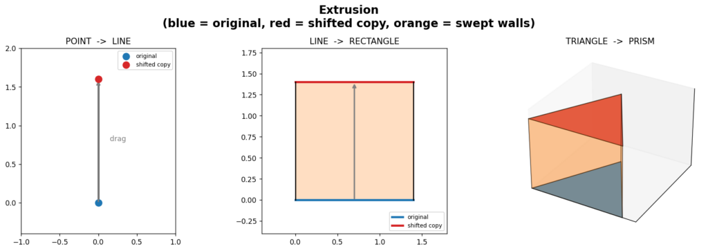
Figure 1: explain extrusion in 1D, 2D, and 3D respectively.

Every rung of that ladder climbs one dimension. The secret is the direction you drag: as long as it points along a fresh axis the shape wasn’t already using, you gain a dimension. Drag a cube in a direction perpendicular to width, height, and depth all at once — a direction we can’t even point at and we’vejust built a shape in 4D.

Slicing: peeking a dimension down

Slicing is the opposite move. Instead of building up, we cut across. Pass a flat plane through a solid, and where it cuts, you get a cross-section one dimension lower. Slice an 2D triangle, you get a line segment; slicing a 3D cube, you will get a 2D square (see figure 2).
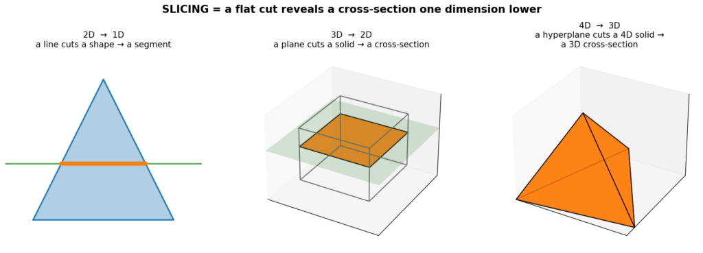
Figure 2: explain slicing in 2D, 3D, and 4D respectively. orange represent the cross-section.

Now push that one rung higher: if we slice a 4D object with a “flat 3D plane” (a hyperplane), and the cross-section is a 3D shape, and this is finally something we can look at. That’s the whole idea. We can’t see the 4D object directly, but we can see its 3D slices.

Putting it together: watching 4D

So here’s how we can actually “see” 4D object in our 3D world. We take a 4D objects and we slice it (1 dimension down). One slice gives one 3D snapshot. But a single snapshot isn’t enough to feel a 4D shape, so we do something more: we slowly rotate the object through the fourth dimension and re-slice it at every step.
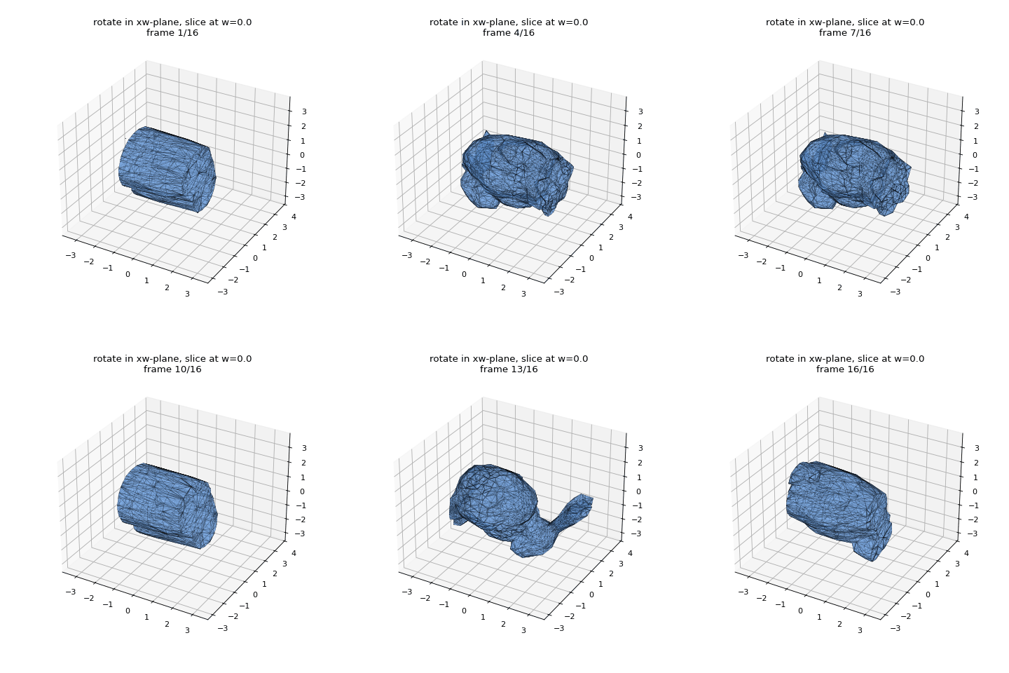
Figure3: Each frame is a single 3D cross-section of a 4D object at fixed w. This mesh is the standford bunny.

Here’s exactly what you’re looking at, step by step:

  1. The object is 4D version of the stanford bunny. Every one of its points has four coordinates: the usual x, y, z, plus a fourth one we’ll call w. We can’t display it directly, because w points in a direction our world doesn’t have.
  2. We fix w and take the cross-section. Holding w at a single value, we ask: which parts of the object live exactly there? That set of points forms a 3D shape — one slice. This is the slicing operation, applied to every little piece of the object and stitched together into the shape you see.
  3. We rotate in 4D. Between frames, we turn the object by a small angle in a plane that involves w (here, the xw-plane). This is a true four-dimensional rotation, and it tips parts of the object that were “elsewhere along w” toward our fixed slice.
  4. We re-slice, and repeat. Because the rotation carries new material through the slice, each frame’s 3D cross-section differs from the last. Play the frames in sequence and the shape appears to be growing, shrinking, splitting, and merging.

And this is the whole magic trick: we use extrusion to build a 4D object from 3D object then slicing to see it. Two simple moves and now a dimension we were never supposed to be able to view suddenly becomes something we can sit back and watch.

References

[1] Alvin Shi, Haomiao Wu, and Theodore Kim. 2025. Hyper-Dimensional Deformation Simulation. In ACM SIGGRAPH 2025 Conference Papers. ACM. https://doi.org/10.1145/3721238.3730730

Categories
Research

3D Object Reconstruction using 2D Medial Axis

During Week 3, we had the incredible opportunity to dive into an amazing project on 3D object reconstruction using medial axis. This journey wouldn’t have been possible without the guidance of Professor Kathryn Leonard and Professor Geraldine Morin. They were truly wonderful advisors, offering us their insight and support every step of the way. We’re so excited to share our thoughts and results with you all! Let’s start with some basic background.

by Stephanie Jung, Evelyn Zhu and Anja Milutinović
  • What is a Medial axis ?

The medial axis is the “skeleton” of a shape. In 2D, the medial axis of a shape is the set of all points that are equidistant from at least two points on the boundary, i.e. the centers of the largest circles you can inscribe inside it. Paired with the radius at each point, it’s a compact yet near-complete description of a shape: sweeping those inscribed disks/balls back along the axis reproduces the original subject. For a straight rod, the medial axis is a line, for a bent tube it’s a curve, and for a torus it’s a circle. The axis really captures a shape’s essential structure in far fewer numbers than the full surface. 

One of the nice properties of the medial axis is that it preserves topology and geometry of the original shape. Given the medial axis of a 2D shape and the corresponding radius of each medial axis point, the original shape can be reconstructed.

  • How do we Compute Medial axis using Voronoi diagrams?

The medal axis is defined with respect to the continuous boundary of a shape and computing exact medial axis is then difficult. It’s then easier to approximate it using Voronoi diagrams of sample points on the boundary.

If we have a set of sample points P = {p1, p2, … , pn}, the Voronoi cell of the sample point pi is a set of all points that are closer to pi, then any other pj:

Vi={x∈ℝn|‖x−pi‖≤‖x−pj‖, ∀j}V_i = \left\{ x \in \mathbb{R}^n \;\middle|\; \|x – p_i\| \le \|x – p_j\|,\ \forall j \right\}

The Voronoi diagram is a collection of all Voronoi cells.

The medial axis and Voronoi diagram’s edges both have in common that they are defined by points that are equidistant from multiple boundary locations. The algorithm to compute medal axis then becomes:

  1. Sample the boundary of the given object
  2. Construct the Voronoi diagram of the sample points
  3. Keep only the Voronoi vertices that are inside the object
  4. Connect the neighboring vertices with existing Voronoi edges
A visual example showing the medial axis of a 2D Baymax silhouette. This particular image actually shows a faulty medial axis. Based on the definition of medial axis, you can determine visually which branches should not be there.

With this foundational understanding of medial axes and Voronoi diagrams under our belts, we were ready to tackle the core of our Week 3 project. We wanted to see if we could take these 2D ‘skeletons’ and use them to solve a much more complex problem: bringing flat images to life by reconstructing a full 3D object from them.

Reconstructing 3d object from its 2d images using medial axis

Method 1:

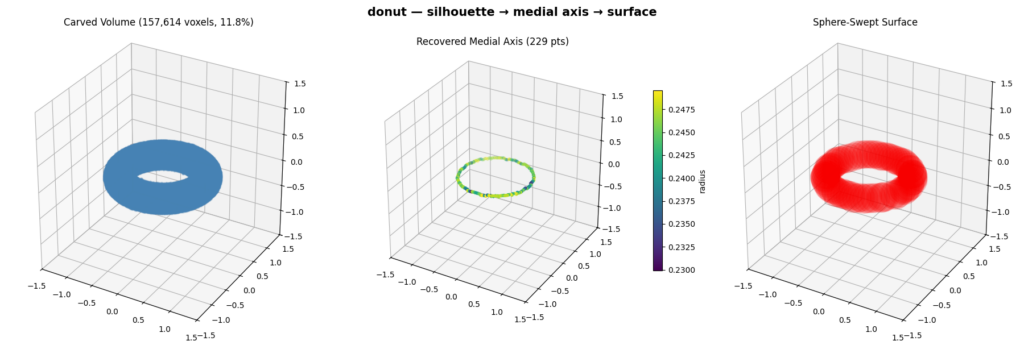
  • We reconstruct a 3D object from a set of binary silhouettes taken from viewpoints spread over a sphere. For each view we compute an orthographic projection of the mesh to get a silhouette, then extract its 2D medial axis and radius via the Voronoi diagram of the boundary. We then fuse the views in 3D by carving a voxel grid (keeping only voxels whose projection lands inside every silhouette) and thin the result with a 3D skeletonization to recover the object’s 3D medial axis. Finally, we rebuild the surface by sweeping balls of the recovered radius along that axis, which reproduces the original shape. 

Pipeline Visualization:

Method 2:

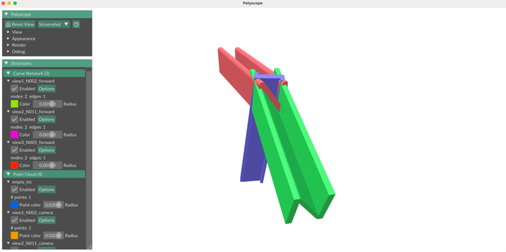
  • Each point on a 2D medial axis represents the center of a maximal inscribed circle. All of the possible centers lie along the camera’s viewing direction. So then, every circle naturally defines a cylinder in 3D space whose axis is the same direction as the camera viewing direction and whose radius equals the radius of the medial circle. Each orthographic image generates an entire set of cylinders, or as we called them “swept cylinders”.
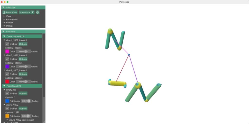
  • We position the “swept cylinders” by setting the medial axis from each camera view in a world space and using the camera parameters (orthographic scale, location with respect to the object, viewing direction) to position each 2D medial axis about the world origin such that it reflected the camera view about the original 3D object. 
N model: Medial axes from 3 different camera views, projected into a world space. Line propagating from the center of each camera view indicates camera forward direction. Blue point (where all camera forwards intersect) indicates the point all cameras were focused on (center of the original 3D object).
N model: Visualization of swept cylinders.

Intersecting the “sweep cylinders” from multiple views in 3D space, gives us a feasible reconstruction region:

Ω=⋂swept cylinders(⋃cylinders in swept cylinderC)\Omega = \bigcap_{\text{swept cylinders}} \left( \bigcup_{\text{cylinders in swept cylinder}} C \right)

Method 2a:

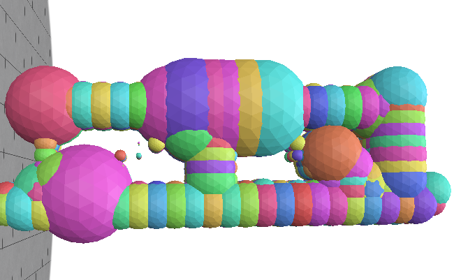
To compute the radii of each sphere we use a signed distance function for a cylinder. Since the center point can belong to multiple cylinders, in each “swept cylinder”, we take the one where the point has a maximum SDF. The sphere must be contained in the intersection of each chosen “swept cylinder”, so the final radius is taken as minimum.

R(p)=minswept cylinders⁡(maxcylinders in swept cylinder⁡SDF⁡(c,p))R(p)=\min_{\text{swept cylinders}} \left( \max_{\text{cylinders in swept cylinder}} \operatorname{SDF}(c,p) \right)
One of the view of the object with it’s 2d medial axis
Reconstruction using maximal spheres with sampled sphere centers

Method 2b:

In an alternative method, to compute the radii of each sphere we use the signed distance field of the binary image for each view, which evaluates a point’s distance from the nearest boundary of the shape. We sample points in 3D space at regular intervals and project them down into each view’s 2D image plane, then compute the signed distance for the point in that view. This method is functionally equivalent to using a 3D signed distance field in world space; it evaluates a point’s distance from the nearest boundary of the swept cylinder for that camera view. Then, the radius of a sphere centered at a point is the minimum signed distance across all camera views, since the sphere must be contained in the intersection of all swept cylinders.

N model (3D)
N model: binary image of the N model from one camera view
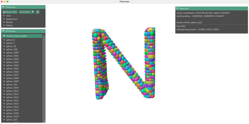
N model: Reconstruction of N model, from images taken from 3 different camera views