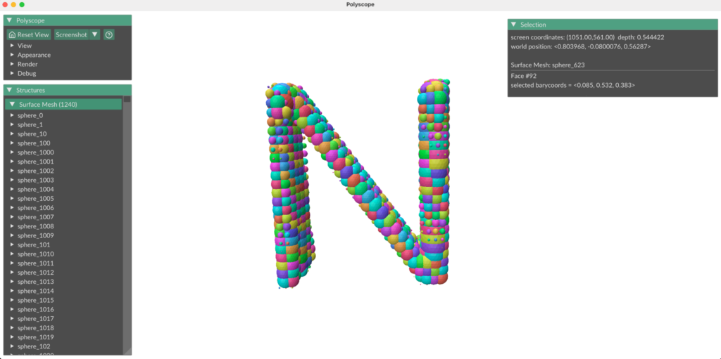
During Week 3, we had the incredible opportunity to dive into an amazing project on 3D object reconstruction using medial axis. This journey wouldn’t have been possible without the guidance of Professor Kathryn Leonard and Professor Geraldine Morin. They were truly wonderful advisors, offering us their insight and support every step of the way. We’re so excited to share our thoughts and results with you all! Let’s start with some basic background.
by Stephanie Jung, Evelyn Zhu and Anja Milutinović
- What is a Medial axis ?
The medial axis is the “skeleton” of a shape. In 2D, the medial axis of a shape is the set of all points that are equidistant from at least two points on the boundary, i.e. the centers of the largest circles you can inscribe inside it. Paired with the radius at each point, it’s a compact yet near-complete description of a shape: sweeping those inscribed disks/balls back along the axis reproduces the original subject. For a straight rod, the medial axis is a line, for a bent tube it’s a curve, and for a torus it’s a circle. The axis really captures a shape’s essential structure in far fewer numbers than the full surface.
One of the nice properties of the medial axis is that it preserves topology and geometry of the original shape. Given the medial axis of a 2D shape and the corresponding radius of each medial axis point, the original shape can be reconstructed.
- How do we Compute Medial axis using Voronoi diagrams?
The medal axis is defined with respect to the continuous boundary of a shape and computing exact medial axis is then difficult. It’s then easier to approximate it using Voronoi diagrams of sample points on the boundary.
If we have a set of sample points P = {p1, p2, … , pn}, the Voronoi cell of the sample point pi is a set of all points that are closer to pi, then any other pj:
The Voronoi diagram is a collection of all Voronoi cells.
The medial axis and Voronoi diagram’s edges both have in common that they are defined by points that are equidistant from multiple boundary locations. The algorithm to compute medal axis then becomes:
- Sample the boundary of the given object
- Construct the Voronoi diagram of the sample points
- Keep only the Voronoi vertices that are inside the object
- Connect the neighboring vertices with existing Voronoi edges

With this foundational understanding of medial axes and Voronoi diagrams under our belts, we were ready to tackle the core of our Week 3 project. We wanted to see if we could take these 2D ‘skeletons’ and use them to solve a much more complex problem: bringing flat images to life by reconstructing a full 3D object from them.
Reconstructing 3d object from its 2d images using medial axis
Method 1:
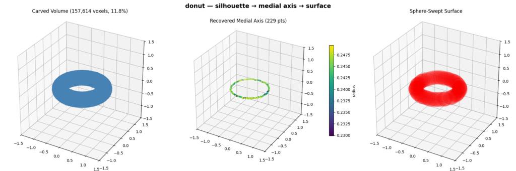
- We reconstruct a 3D object from a set of binary silhouettes taken from viewpoints spread over a sphere. For each view we compute an orthographic projection of the mesh to get a silhouette, then extract its 2D medial axis and radius via the Voronoi diagram of the boundary. We then fuse the views in 3D by carving a voxel grid (keeping only voxels whose projection lands inside every silhouette) and thin the result with a 3D skeletonization to recover the object’s 3D medial axis. Finally, we rebuild the surface by sweeping balls of the recovered radius along that axis, which reproduces the original shape.
Pipeline Visualization:

Method 2:
- Each point on a 2D medial axis represents the center of a maximal inscribed circle. All of the possible centers lie along the camera’s viewing direction. So then, every circle naturally defines a cylinder in 3D space whose axis is the same direction as the camera viewing direction and whose radius equals the radius of the medial circle. Each orthographic image generates an entire set of cylinders, or as we called them “swept cylinders”.
- We position the “swept cylinders” by setting the medial axis from each camera view in a world space and using the camera parameters (orthographic scale, location with respect to the object, viewing direction) to position each 2D medial axis about the world origin such that it reflected the camera view about the original 3D object.
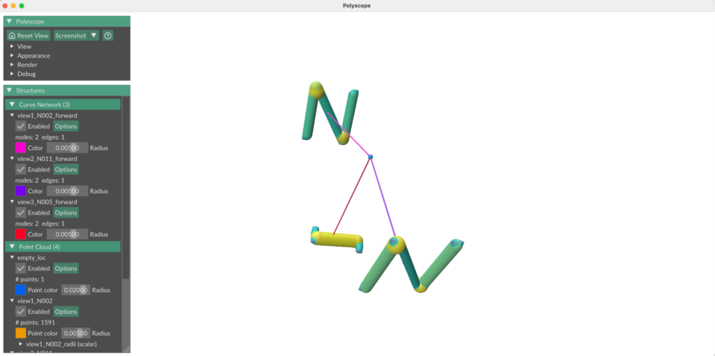
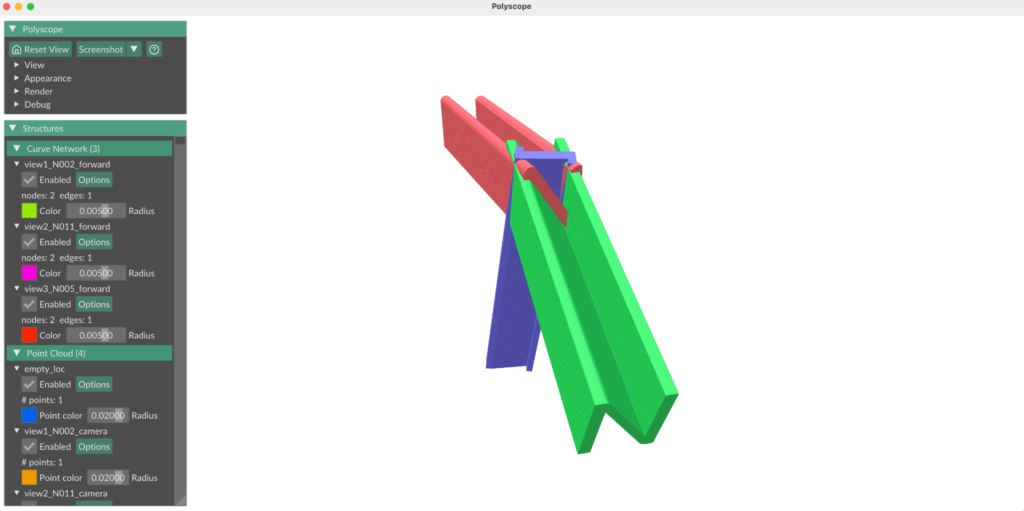
Intersecting the “sweep cylinders” from multiple views in 3D space, gives us a feasible reconstruction region:
Method 2a:
To compute the radii of each sphere we use a signed distance function for a cylinder. Since the center point can belong to multiple cylinders, in each “swept cylinder”, we take the one where the point has a maximum SDF. The sphere must be contained in the intersection of each chosen “swept cylinder”, so the final radius is taken as minimum.

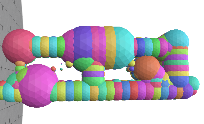
Method 2b:
In an alternative method, to compute the radii of each sphere we use the signed distance field of the binary image for each view, which evaluates a point’s distance from the nearest boundary of the shape. We sample points in 3D space at regular intervals and project them down into each view’s 2D image plane, then compute the signed distance for the point in that view. This method is functionally equivalent to using a 3D signed distance field in world space; it evaluates a point’s distance from the nearest boundary of the swept cylinder for that camera view. Then, the radius of a sphere centered at a point is the minimum signed distance across all camera views, since the sphere must be contained in the intersection of all swept cylinders.