Self-Rectifying Textures

By: Kyle Loh, Mahlet Girma, Max Dunitz

If you have ever had to flatten out a bag of chips so the checkout scanner would finally read it, you already understand the problem we worked on this week. A code printed on a surface that bends, folds, or curves is hard to read, and QR codes and barcodes carry one disadvantage here: they are obvious. In supply-chain tracking, that single visible code can be tampered with, causing a product to be moved into a market it was not meant for. Our project examines self-rectifying textures, which are patterns that look like random noise, but their autocorrelation contains a regular lattice. By measuring how that lattice bends in a photo, we can recover how the surface was deformed, without printing a single visible marker.

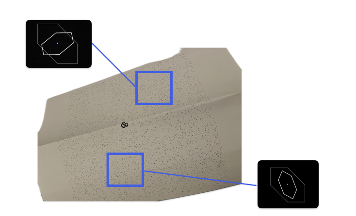
The usual way to undo a perspective distortion is to find distinct points (for example, the three eyes of a QR code) and use their pixel positions to solve for a homography. To stay hidden, self-rectifying textures move the landmarks into the autocorrelation of the image.

Definition of Autocorrelation: The autocorrelation measures how much an image resembles a shifted copy of itself. It is basically a dot product. For a 2D image $f: \mathbb{R}^2 \rightarrow \mathbb{R}$, the autocorrelation is defined as follows:

where $x$ is a pixel position and the lag (or shift) $\tau \in \mathbb{R}^2$. A peak is defined as the $\tau$ where $R_{f,f}(\tau)$ attains a local maximum. This operation is translation-invariant.

As autocorrelations are computationally expensive $(\mathcal{O}(N^2))$, we never compute them directly. Instead, we invoke the Wiener-Khinchin theorem, allowing us to compute the autocorrelation in terms of Fourier transforms ($\mathcal{F}$): $R = \mathcal{F}^{-1}(|\mathcal{F}(f)|^2)$ in $\mathcal{O}(N\log N)$.

Task 1 – Constructing Textures: We used a grayscale-version of Steamboat Willie with a fronto-parallel view as our base image.

Next, we superimposed three copies of the image, each offset by shift vectors $0, +u, +v \in \mathbb{R}^2$, using zero-padding. We call the superimposed image the base texture. The following autocorrelation plot would have six peaks, at $\{ \pm u, \pm v, \pm (u-v)\}$. This is known as the Fundamental Hexagon. Then, we apply a deformation $A$ to the superimposed image, causing the fundamental hexagon to become $\{ \pm Au, \pm Av, \pm A(u-v)\}.$

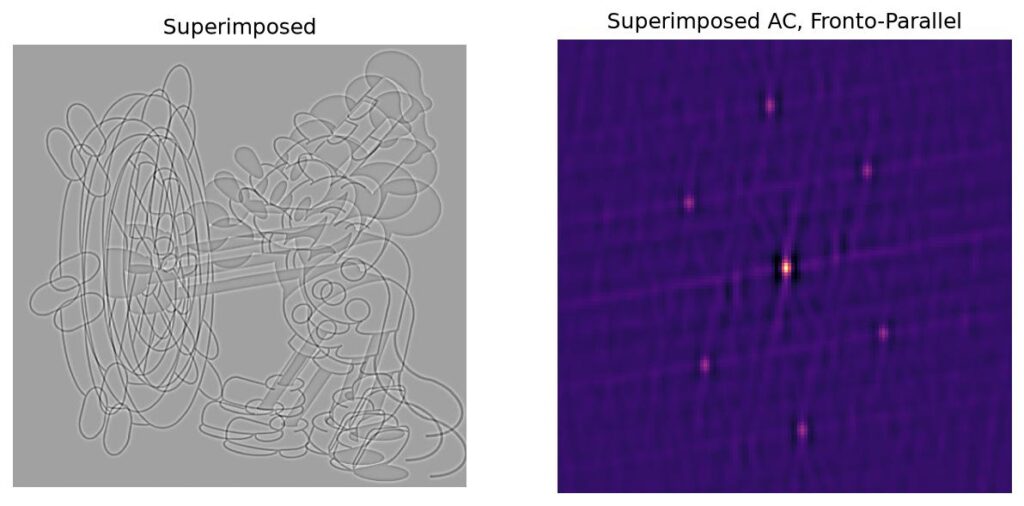
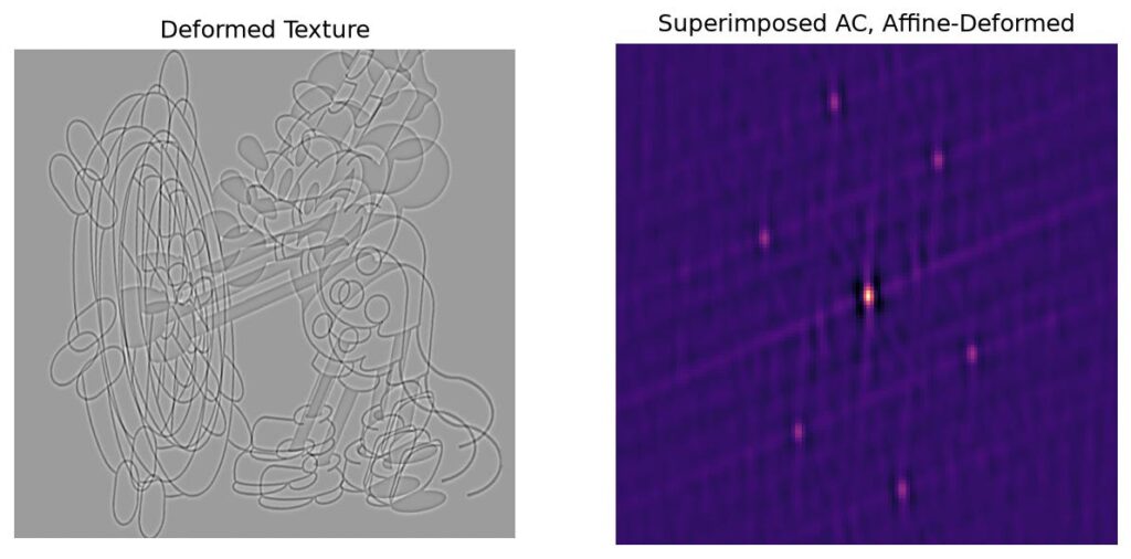
The Assignment Problem: Suppose you know the original shifts $\{ \pm u, \pm v, \pm (u-v)\}$ and have access to the base texture, but not the deformation. Unfortunately, the deformed hexagon $\{ \pm Au, \pm Av, \pm A(u-v)\}$ alone does not tell you which peak corresponds to $Au$ and which to $Av$, or their signs. However, if you can figure out this assignment problem, then you can immediately solve for $A$ with some linear algebra.

Given the symmetries, there are eight sign-and-order combinations. Using certain invariance properties, this can be reduced to six combinations. We find and apply six candidate inverse maps $A^{-1}$ and select the inverse map with the highest normalized cross-correlation score against the base texture. This is a computationally expensive solution, and for future work, we will explore more efficient methods for the assignment problem.

Task 2 – Full Rectification Pipeline: We introduce a method that no longer assumes a uniform linear deformation. Our goal is to recover a global inverse map $\phi^{-1}$ that maps the observed texture back to a fronto-parallel image.
For this experiment, we used blurred Gaussian white noise as our base image, constructing a texture by superimposing it with two shifted copies of itself and zero-padding. We then apply a homography deformation $A$.

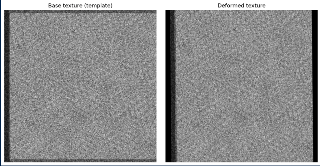
Methodology: We sample small square patches from the grid. Then, we compute each patch’s autocorrelation and patches with “unreliable measurements” are discarded — criteria include: no valid fundamental hexagon detected or the inverse Jacobian’s determinant is a statistical outlier). For each patch, we detect the warped fundamental hexagon in each patch’s autocorrelation. Comparing these peaks with the known original shifts provides six candidates for the local inverse Jacobian $D\phi^{-1}(y_i)$.

Then, we construct a Delaunay triangulation mesh of the center points of the remaining patches. Two measurements are treated as neighbors when their centers share an edge in the mesh. To select on candidate Jacobian at each vertex, we assume that the physical deformation varies smoothly, so the correct matrices at neighboring vertices should be similar.

We resolve the candidate ambiguity using Minimum Spanning Tree propagation. First, we use a phase correlation on one patch with the original template to select one initial vertex and its actual local Jacobian $D\phi^{-1}(y_i)$. Suppose vertex $i$ has been already assigned the matrix $G_i^\ast$ while an adjacent vertex $j$ remains unassigned. For each of the six candidates at $j$, we compute the mismatch

and take the candidate with the minimum Frobenius norm. All edges from assigned vertices to unassigned vertices are stored in a priority queue, and we iteratively assign matrices to unassigned vertices adjacent to vertices with assignment.
Finally, we use a finite-element method that reconstructs a global inverse map whose gradient best matches the selected local Jacobians:

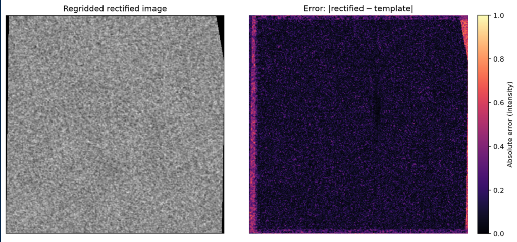
This determines the map up to a constant translation (the +C in integration), so we anchor the reconstructed mesh to the image boundary. We then regrid the deformed pixel values through the recovered map to produce a rectified image. For validation, we compare this result with the original template using the absolute error $|rectified – template|$.

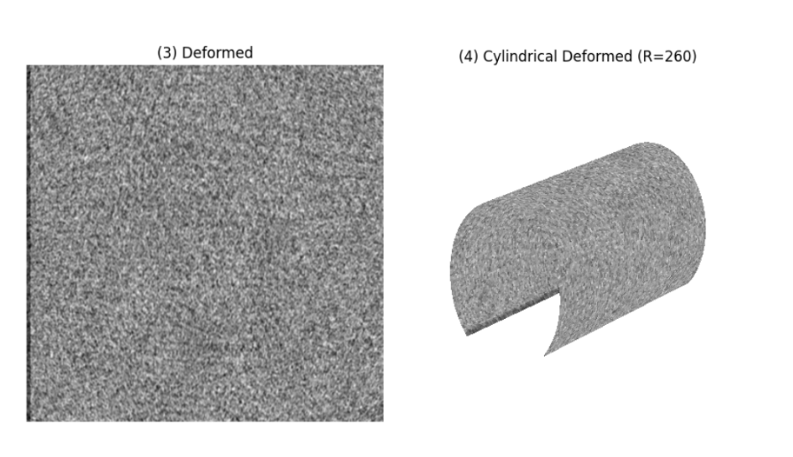
Task 3 – Non-Planar Texture Rectification via Cylindrical Mapping: We extend our rectification pipeline to non-planar surfaces (particularly, a homography-deformed white-noise texture wrapped around a cylinder) utilizing the same MST and Finite Element Method pipeline from Task 2 to recover a global inverse deformation map.

Note: To model deformations on cylindrical geometry, spatial coordinates $(X,Y)$ in the planar texture domain are mapped to 3D surface coordinates $(X,Y, Z)$ for a cylinder of radius R=260px. To unroll or warp texture fields back into the reference domain, we map the angular coordinates $\theta = \text{atan2}(Y,X)$ back into 2D planar coordinates $(X,Y)$.

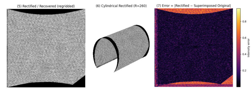
Conclusion: Our rectification pipeline has a clear strength: most internal vertices (from the Delaunay triangulation) have sub-pixel error in the rectification and are accurate intensity-wise. However, the pipeline also has two clear weaknesses: (1) there are larger intensity errors at the edges and corners, most likely from our failure to collect as many “good” observations near the edges and corners of the texture and (2) the dependency on accessing the template at least once in the process. Future work would entail resolving these two issues.

References:
[1] Bencheikh, Ismail, et al. “Autocorrelation-based Fiducial Markers for Traceability.” Proceedings of the IEEE/CVF Winter Conference on Applications of Computer Vision. 2026.