Exploring Dependence Between Curvature and Heat Diffusion on a Mesh

By Shannon Cudworth, Mentors: Alek Fröhlich and Daniel Perazzo

Introduction

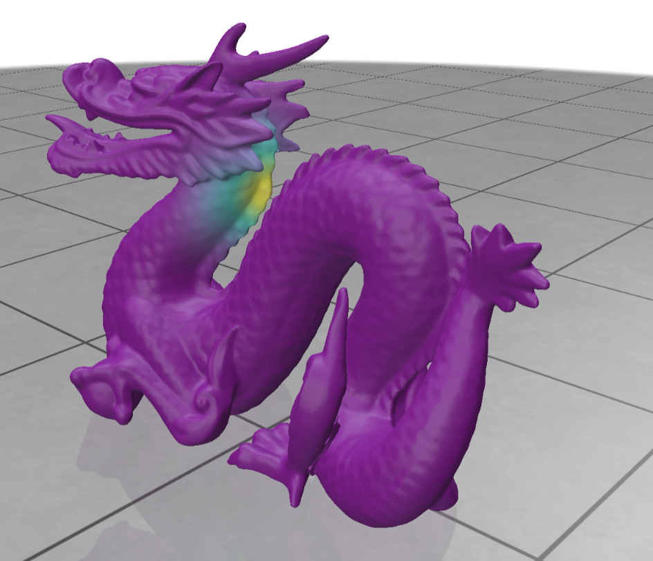
The goal of the project was to study statistical dependence from geometric perspective, where we define two random variables X, Y are defined on a surface $\mathcal{M}$ , rather than in a Euclidean space. Specifically, we explore whether heat diffusion across a surface is dependent on the local curvature.

To study this relationship, we randomly sample a triangle face from a mesh and then construct one heat diffusion variable and one curvature variable for this sampled face. The former variable was defined using the Laplace-Beltrami operator, and for the latter variable we used the mean curvature value at the sampled face’s barycenter. We then employed the Hilbert–Schmidt Independence Criterion (HSIC) to investigate if faces with similar heat diffusion also have similar curvature.

To implement, we first sample faces with a probability proportional to their area, to avoid oversampling smaller triangles. After constructing the two aforementioned variables, we make curvature and heat kernel matrices to describe pairwise curvature and heat similarity, run a permutation test, and repeat for various sample sizes to estimate the power of the sample HSIC test.

Constructing the Heat Diffusion Variable

To approximate heat diffusion, we’re going to use the Laplace-Beltrami operator. For this, we need the cotangent Laplacian and mass matrix.

Cotangent Laplacian: A discrete approximation of the Laplace-Beltrami operator, used on triangle meshes. We define this matrix using the piecewise function:

L_{ij} = \begin{cases} -\frac{1}{2}\left(\cot\alpha_{ij}+\cot\beta_{ij}\right), & i\neq j,\ (i,j)\in E,\\ \sum_{k\in\mathcal{N}(i)} \frac{1}{2}\left(\cot\alpha_{ik}+\cot\beta_{ik}\right), & i=j,\\ 0, & \text{otherwise.} \end{cases}

Where $\alpha_{ij}$ and $\beta_{ij}$ are opposite angles for the edge (ij), and N(i) is the set of neighboring vertices to vertex i.

Mass Matrix: Represents how much of the mesh’s surface area is associated with each individual vertex, and was defined using gpy toolbox.

With both of these components, we can understand the geometric variation of the mesh’s surface (through the Laplacian), and how much the variation contributes to the overall surface area of the mesh (though the Mass Matrix).

To actually approximate the heat diffusion over the area, we need to solve the eigenvalue problem:

L\phi_i = \lambda_iM\phi_i

where L is the cotangent laplacian, M is the mass matrix, $\phi_i$ is the ith eigenvector, and $\lambda_i$ is the corresponding ith eigenvalue.

Using Scipy, we solve for the first 100 eigenvector-eigenvalue pairs, which represents the 100 smoothest solutions to the equation above. The eigenvector defines a basis function over the mesh vertices, and the eigenvalue is the rate of decay under heat diffusion.

Now, to construct our random variable X, we must recall that we have sampled a random face of the triangle mesh, and we have two arrays eigenvectors and eigenvalues, where:

eigenvectors[i]
eigenvalues[i]

returns the first 100 eigenvectors and eigenvalues at vertex i of the mesh. To utilize these arrays, we must directly evaluate the eigenvalue problem at the sampled face’s barycenter. Then for the sampled face with vertices i,j,k we calculate:

(eigenvectors[i] + eigenvectors[j] + eigenvectors[k]) / 3

which gives us a vector of the form:

\begin{bmatrix} \phi_1(b_i) \\ \phi_2(b_i) \\ \vdots \\ \phi_{100}(b_i) \end{bmatrix}

where $b_i$ is the barycenter of the ith sampled face.

Then using the respective eigenvalue, we can construct a random variable $X_i$ that represents the heat diffusion from barycenter of the ith sampled face with:

X_i = \begin{bmatrix} e^{-t\lambda_1/2}\phi_1(b_i) \\ e^{-t\lambda_2/2}\phi_2(b_i) \\ \vdots \\ e^{-t\lambda_{100}/2}\phi_{100}(b_i) \end{bmatrix}.

**Figure:** Heat diffusion from the barycenter of the sampled face on the dragon mesh

Constructing the Curvature Variable

To construct the curvature variable, we calculate the mean curvature at each of the sampled face’s three vertices. Using libigl’s principal curvature value function, we return $k_1, \space k_2,$ the maximum and minimum curvature values at a vertex, respectively. We can then calculate the mean curvature value, defined as:

H = \frac{(k_1 + k_2)}{2}

If the mean curvature is small or 0, we can interpret either a locally flat surface, or a saddle structure where $k_1$ and $k_2$ cancel each other out. A larger mean curvature indicates bending.

Then for the ith sampled face with vertices i,j,k, we can construct the random variable $Y_i$ , which will calculate the curvature at the face’s barycenter, defined as:

Y_i = H(b_i) = \frac{(H_i + H_j + H_k )}{3}

where $H_i,\space H_j, \space H_k$ are the mean curvature values at vertex i, j, k, and $H(b_i)$ is the mean curvature at the barycenter of the ith sampled face.

Kernels

To check independence between our two random variables X and Y, we must construct kernel matrices, which will measure the similarity between pairs $X_i, \space X_j$ and $Y_i, \space Y_j$ (Schrab 19).

X variable: By construction of the laplacian, we can calculate the heat kernel $K_X$ by:

K_X = XX^T

By definition:

X_i = \begin{bmatrix} e^{-t\lambda_1/2}\phi_1(b_i) \\ e^{-t\lambda_2/2}\phi_2(b_i) \\ \vdots \\ e^{-t\lambda_{100}/2}\phi_{100}(b_i) \end{bmatrix}.

Then we can say for any i,j:

X_{i}X_{j}^{\top} = \sum_{\ell=1}^{100} \left( e^{-t\lambda_\ell/2}\phi_\ell(b_i) \right) \left( e^{-t\lambda_\ell/2}\phi_\ell(b_j) \right)

Then,

X_{i}X_{j}^{\top} = \sum_{\ell=1}^{100} e^{-t\lambda_\ell}\phi_\ell(b_i) \phi_\ell(b_j)

which is the heat kernel formula (Mostowsky et al.).

Y variable: Unlike the heat diffusion variable X, we need to do a few more calculations to compute the curvature kernel $K_Y$ , which we will do by using the Gaussian Kernel formula.

First, we define $\sigma_Y$ , which represents the median pairwise distance for each $Y_i,\space Y_j$ pair. Then we can calculate the kernel $K_Y$ using the formula, for each i,j pair:

K_Y(i,j) = exp(-\frac{||Y_i – Y_j||^2}{2\sigma_Y^2})

If $K_X, \space K_Y$ are large, then it follows that the ith and jth sampled faces have similar diffusion or similar curvature, respectively. Rather, if the kernels are small, then we can say the ith and jth sampled faces have different diffusion or curvature, respectively.

Hilbert-Schmidt Independence Criterion (HSIC)

The kernel matrices $K_X, K_Y$ allow us to determine if there are any similarities between pairs $X_i, \space X_j$ or $Y_i, Y_j$ . Now, we want to examine that if pair $X_i, X_j$ are similar, if it is true that pair $Y_i, Y_j$ are similar as well. To acheive this, we compute the sample HSIC.

To ensure valid comparability between variables, we first make a centering matrix, defined as:

H = I_{nxn} – \frac{1}{n}J_{nxn}

where $J_{nxn}$ is a matrix of all ones.

We can then define the centered kernels for X and Y as:

K_{XC} = HK_xH \\\\\\\\\\\\\ K_{YC} = HK_YH

Then, by definition,

HSIC(K_X,K_Y) = \frac{1}{(n-1)^2}tr(K_{XC}K_{YC})

Here, a large sample HSIC value indicates dependence between heat diffusion and curvature (Schrab 25).

Permutation Testing and Power

One sample HSIC value isn’t enough to statistically determine whether or not X, Y have dependence. So, we must undergo a permutation test. To start, we define a null and alternative hypothesis:

$H_0: X, Y \space are \space independent \\ H_A: X, Y \space are \space dependent$

Our goal for this test is to simulate under the null hypothesis, and then see how likely our originally observed sample HSIC is to occur in those conditions. We permute the order of $K_Y$ , recompute the sample HSIC, and repeat 200 times to create the null distribution. We then use the observed sample HSIC to calculate a p-value, which indicates whether or not we should reject or fail to reject the null hypothesis.

Taking a step further, we calculated the power of the sample HSIC test, which will give us the probability that, when X and Y are dependent, the sample HSIC will correctly detect that dependence. We do this by repeating the permutation test, and dividing the amount of times we rejected the null (p-value was less than 0.05, depending on significance level) by the total amount of retrials.

In our project, we compared the power of the sample HSIC test across sample sizes: 5, 10, 25, 50, 75, and repeated the permutation test 100 times per each sample size. We also compared the sample HSIC using the aforementioned heat diffusion kernel that was calculate with the Laplace-Beltrami operator, and another heat diffusion X variable and kernel, that was constructed using a numerical approximation and Gaussian Kernel method.

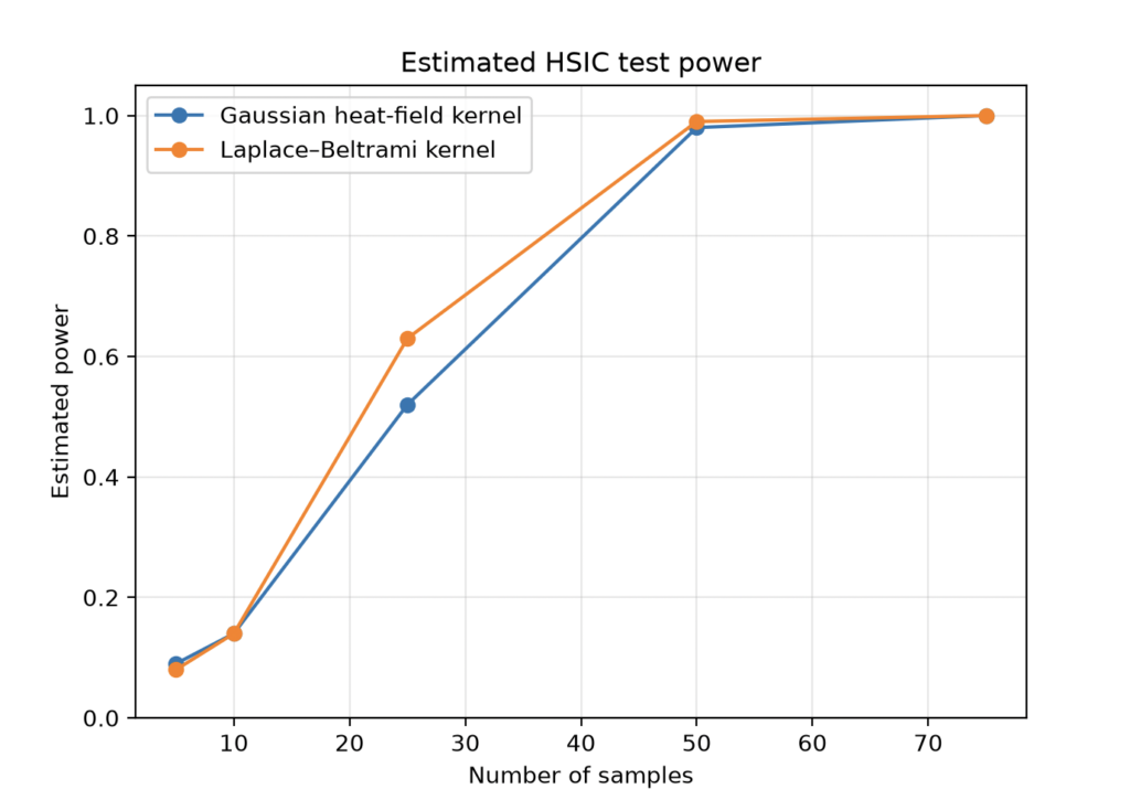
**Figure:** Shows the HSIC test power between random variables X,Y with a Gaussian heat diffusion kernel and Laplace-Beltrami heat diffusion kernel. Note that while the Laplace-Beltrami kernel does better for smaller samples, both converge to 1 as sample size increases.

From the figure, we can see that, as the sample size increases, the power of sample HSIC test equals 1. This means that every trial rejected the null hypothesis, and the sample HSIC test is successful at detecting dependence between heat diffusion and curvature.

Possible Extensions of the Project

I think it would be fun to compare the sample HSIC across different meshes, and maybe how quickly the power of the sample HSIC test converges to one across different meshes. We could also compare different curvature formulas with heat diffusion, or vary the time that we allow heat diffusion to occur. Or, we can explore with different variables, such as letting X represent the geodesic field from a sampled face, and compare that to curvature.

Works Cited

Schrab, Antonin. “Optimal Kernel Hypothesis Testing.” University College London, 2025.

Mostowsky, Peter, et al. “The GeometricKernels Package: Heat and Matérn Kernels for Geometric Learning on Manifolds, Meshes, and Graphs.” Journal of Machine Learning Research, vol. 26, no. 276, 2025, pp. 1–14.

odedstein. sgi-introduction-course. GitHub, https://github.com/ddecatur/sgi-introduction-course.

Author

shannon.cudworth