Surface Log Maps

by Anja Milutinovic and Shannon Cudworth

Geodesics and geodesic distance

Suppose we have a curved surface M⊂$\mathbb{R}^3$. If we want to measure distances or move from one point to another, Euclidean straight lines are no longer appropriate because they leave the surface. So we generalise the notion of a “straight line”, by seeking the straightest possible path that remains on the surface. This is called a geodesic.

More formally, a geodesic is a curve that locally minimizes the length L of the curve:

The geodesic distance between two points p, q M is:

Exponential and logarithmics maps

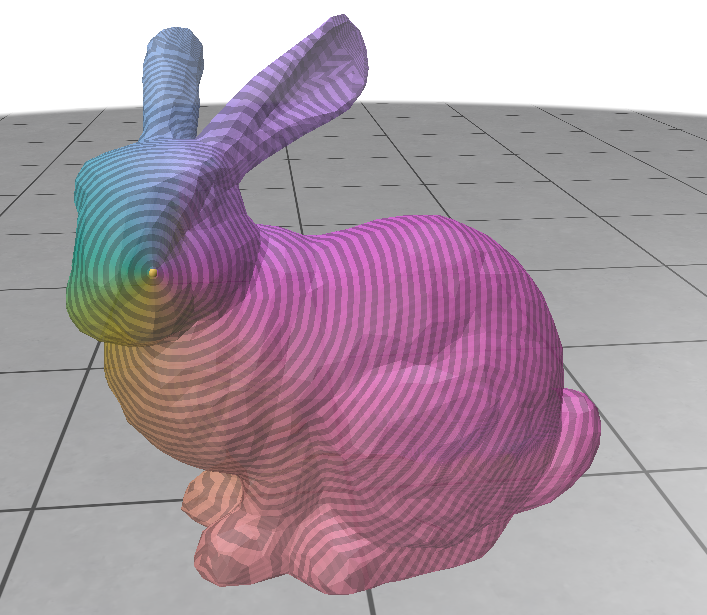
Given a point $p\in M$ and a tangent vector $v\in T_pM$, there exists a unique geodesic $\gamma$ such that $\gamma(0)=p$ and $\gamma'(0)=v$. Exponential map $\operatorname{Exp}_p:T_pM\rightarrow M$ is a map that for every $v\in T_pM$ gives the endpoint of the geodesic starting at p with the direction $v$ and length $\|v\|$. 

Then, the logarithmic map is the inverse of the exponential map,  $\operatorname{Log}_p:M\rightarrow T_pM$, whenever the exponential map is invertible. Logarithmic map for any given point $q\in M$ is a tangent vector that gives the initial direction of a geodesic starting at p and ending at q.

Combining the logarithmic map with the frame $\phi_p:T_pM\rightarrow\mathbb{R}^2$, we get 

$z=\phi_p\circ\operatorname{Log}_p$, that maps any point q on a surface into $\mathbb{R}^2$.

Levi Civita connections

Given two neighboring vertices $v_1, v_2$ on a discrete triangle mesh, we can define corresponding tangent vectors $t_1, t_2,$ such that $t_1$and $t_2$ belong to the tangent planes at $v_1$ and $v_2,$respectively. Since $t_1,\ t_2$ lie on different tangent planes, we cannot meaningfully compare them. Our goal is to define a parallel transport, which moves one tangent vector to another tangent plane at an adjacent vertex, while minimizing rotation, known as the Levi Civita connection.

To implement the Levi Civita connection, we are given a dictionary containing all vertices with a shared edge, and the normal vector defined at every vertex $v_i$. By looping over all shared edges $i,j$, we take neighboring vertices $v_i, v_j$ and we index and define the normal vectors corresponding with the vertices, labeled $n_1$and $n_2$, respectively.  We then use the normals to calculate the Rodrigues Rotation, or the rotation of a vector by a specific angle around a fixed axis. The formula to determine this rotation matrix is given by:

where $v = n1 \times n2,\ c = n1 \cdot n2, \ s = ||v||, \ \mathbf{v}_{\times}=\left[\begin{array}{ccc}0&-v_2&v_1\\v_2&0&-v_0\\-v_1&v_0&0\end{array}\right]$

Then R approximates Levi Civita connection between adjacent tangent planes.

Connection Laplacian

After constructing the Levi Civita connection, we want to compare the tangent vectors at neighboring vertices, which is accomplished through the Connection Laplacian. As before, we loop over all vertices i,j with shared edges, and first define the cotangent weights, which are given by:

where $\alpha_{ij}$ and $\beta_{ij}$ are the two angles opposite the edge (i, j). Now we can define the Connection Laplacian matrix, defined as:

where $w_{ij}$ is the cotangent weight between vertex i and vertex j, $R_{ij}$ is the Levi Civita connection between vertex i and vertex j, and $N(i)$ is the set of adjacent vertices to vertex i. Once the Connection Laplacian is defined, we can now measure how tangent vector fields change across vertices and our mesh.

Heat Diffusion & Vector Heat Method

With the Levi Civita connection and the Connection Laplacian, we can now define the Vector Heat Method (VHM), which approximates parallel transports between arbitrary vertices on our surface.

Given a mass matrix M, a connection laplacian L, an initial vector field V, and a small time step h, we can solve the vector heat equation:

where X is a vector field that approximates the parallel transport of V along the minimal geodesics.

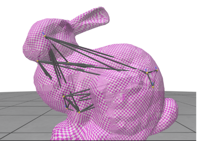
We now introduce a set of user-selected seed vertices S = { $s_1,\ … \ , s_k$ } ⊂V. Via the VHM, we can approximate the parallel transport between any arbitrary seed vertices. Our goal is to extend this to the Affine Heat Method, which will use the VHM estimations of parallel transport between seed frames to optimize a set of tangent frames, allowing adjacent logarithmic maps to be more effectively blended.

Seed graph with optimal frames & UV offset

A single logarithmic map only provides a low-distortion parameterization around one point on the surface. To cover the entire mesh, we choose a small set of seed vertices$$S=\{s_1,\ldots,s_k\}\subseteq V,$$and compute one logarithmic map around each seed. Each seed defines its own local coordinate system describing the nearby geometry.

Since these maps are computed independently, their coordinate systems are arbitrary. Even if two neighboring maps describe the same part of the surface, one may be rotated relative to the other. Before we try to combine the maps, their orientations must be made consistent.

We therefore associate each seed with a local frame $t_s \in T_sM$. Specifically, we define a linear map $\Psi_s : T_sM \rightarrow \mathbb{R}^2$ that maps the local frame to the horizontal axis of the plane.

However, the maps may still be translated.o fix this, we assign each seed a UV offset $w_s\in\mathbb{R}^2$. Neighboring logarithmic maps should predict the same relative displacement, leading to the consistency condition:

he UV offsets are then computed by minimizing the disagreement between neighboring seeds.

Blending seed’s log maps

The final step was to combine the local parameterizations into a single global UV map. This involves deciding which local maps influence each part of the surface and how they should be combined. One way to this is to partition the surface into Voronoi cells, where each vertex is assigned to its nearest seed according to geodesic distance and inherits that seed’s local parameterization. While this approach is simple and efficient, it creates visible seams at the boundaries between neighboring cells.