One may think that the order in which an algorithm processes geometric data should not affect its result. Consider simplifying a triangular mesh by repeatedly collapsing edges. The mesh contains the same numbers of vertices, edges, and faces. The simplification also targets the same final edge count, so one might expect approximately the same amount of computation. In practice, however, layout can significantly affect runtime.
For example, in our experiments, the three locality-aware ordering methods that we tested reduced edge-collapse time by up to 18%.
Processors rely on caches, which are small, fast stores for recently accessed data. If required data is already cached, it can be retrieved quickly; otherwise, the processor must retrieve it from slower main memory, causing a cache miss. An edge collapse accesses the faces, edges, and vertices surrounding the selected edge. When neighboring elements are stored close together in memory, the processor has more opportunities to reuse cached data. When they are scattered, those opportunities decrease, which can increase cache misses and slow the algorithm.
We investigated this effect onlamppost.obj, comparing a randomized ordering baseline against three locality-aware strategies that we re-implemented (Morton ordering [1], Hilbert ordering [2], and Tipsify [3]).
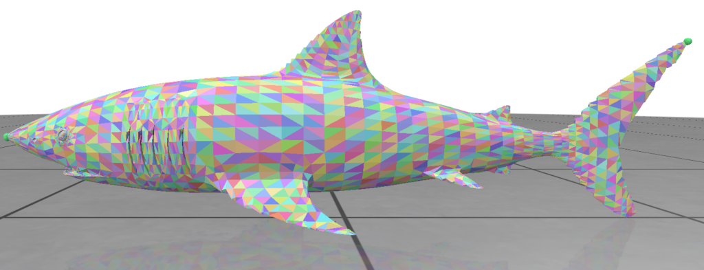
The same connected triangle group is highlighted under random and Morton orderings. Random ordering scatters these faces throughout the face array, with vertices ranging 184,989 indices, whereas Morton ordering places them in a more compact interval with vertices ranging 303 indices.
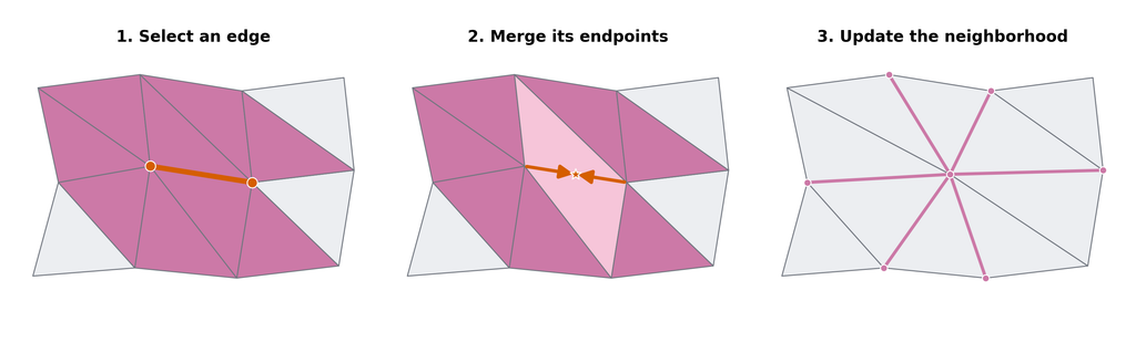
Edge Collapse: Edge collapse is an operation for reducing the complexity of a triangle mesh [4]. Given an edge connecting two vertices, the operation effectively merges its endpoints and removes triangles that become degenerate. Repeating this process reduces the number of vertices, edges, and faces while approximately preserving the original surface.
Figure 2: Three stages of an edge collapse: (1) selecting an edge and its local neighborhood, (2) merging the edge’s endpoints, and (3) updating the resulting connectivity.
Our implementation uses CGAL’s Surface Mesh Simplification package, whoseedge_collapse algorithm iteratively collapses edges until a user-provided stopping condition is satisfied [5]. Each collapse requires information about the selected edge’s neighborhood. In particular, the algorithm accesses the endpoints, adjacent triangles, and nearby edges. Reordering the mesh attempts to assign nearby indices to elements that are likely to be accessed together, increasing the chance that their data remains available in cache.
Methods: We introduce the three locality-aware methods for re-ordering triangles/vertices in a mesh: Morton, Hilbert, and Tipsify. After re-ordering the mesh using these three methods, we compare the runtimes of the edge collapse algorithm on the re-ordered mesh against the mesh generated from randomly ordered vertices.
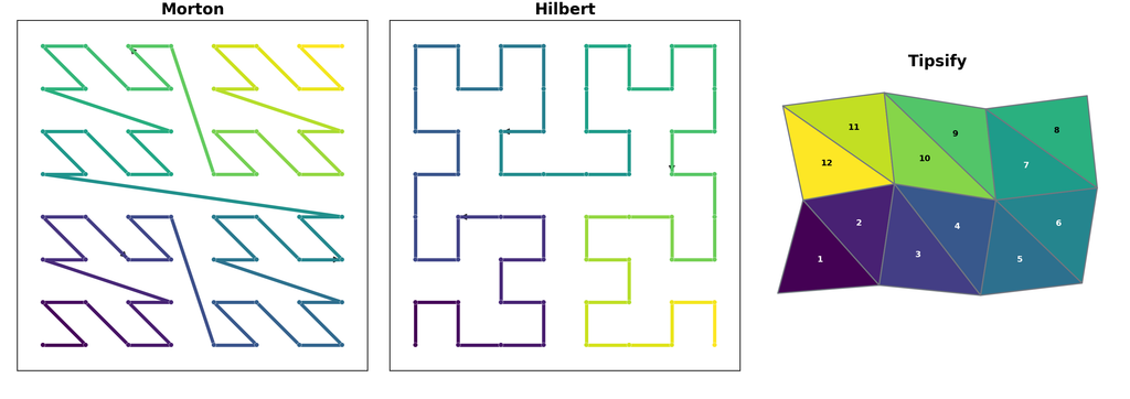
Figure 3: Small 2-dimensional example with (a) Morton ordering; (b) Hilbert ordering; (c) Tipsify ordering.
Morton Sorting: Morton sorting orders triangles according to the positions of their centroids by assigning them a binary number known as the key. The procedure is as follows: 1. Compute the mesh’s bounding box, which is the smallest box containing the entire mesh. 2. Divide the bounding box in half along all three coordinate axes, producing eight smaller boxes called octants. 3. Determine which octant contains each triangle’s centroid and record that octant (after encoding into bits) as the first part of the triangle’s key. 4. Divide the selected octant into eight smaller octants and again record which one contains the centroid. 5 . Repeat this subdivision to the desired level of precision. The resulting sequence of octants forms the key for each triangle. 6. Sort the triangles by their key. Since triangles in the same region begin with similar keys, this tends to place spatially nearby triangles close together in the face array.
Hilbert Curve Sorting: Hilbert sorting also orders triangles according to the positions of their centroids. Like Morton sorting, it repeatedly divides the mesh’s bounding box into octants. The difference is that it visits the octants along a continuous path. The procedure is as follows: 1. Compute the mesh’s bounding box and divide it in half along all three coordinate axes, producing eight octants. 2. Visit the eight octants in an order that moves between adjacent regions. 3. Determine which octant contains each triangle’s centroid and record its position in the traversal as the first part of the triangle’s Hilbert key. 4. Divide each octant into eight smaller octants and repeat the traversal inside it. 5. Rotate or reflect each smaller traversal so that it connects continuously to the regions visited immediately before and after it. 6. Continue subdividing to the desired level of precision. The resulting sequence of visited regions forms a Hilbert key for each triangle. 7. Sort the triangles by their Hilbert keys. Since consecutive portions of the traversal usually correspond to neighboring regions, this tends to place spatially nearby triangles close together in the face array.
Tipsify: Unlike Morton and Hilbert curves, Tipsify does not consider triangle centroid location and looks instead at which triangles share vertices. It walks across the mesh one triangle at a time while keeping track of a small list of the most recently used vertices as well as vertex-to-triangle adjacencies. The traversal proceeds as follows: (1) For every vertex, record the triangles incident to it and count how many of those triangles have not yet been added to the reordered triangle list. (2) Choose a current vertex. Add each of its unprocessed incident triangles to the reordered triangle list. Whenever a triangle is added, update the number of unprocessed triangles remaining at each of its vertices and update the simulated vertex-cache state. (3) From the vertices belonging to the newly added triangles, choose a vertex from which to continue. Prefer a vertex that still has unprocessed incident triangles and is predicted to remain in the simulated cache while those triangles are processed. (4) If no suitable nearby vertex remains, search recently encountered vertices for one that still has unprocessed incident triangles. If none exists, scan the remaining vertices until such a vertex is found. (5) Repeat until every triangle has been added exactly once. The order in which the triangles were added becomes the new triangle order.
Remark: While Hilbert and Morton sortings were designed for CPU caches, Tipsify was originally designed for GPU caches. Here, we test whether Tipsify’s connectivity-aware triangle order also benefits a CPU edge-collapse implementation.
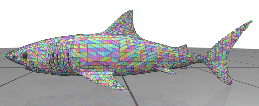
Figure 4: The lamppost mesh under random, Morton, Hilbert, and Tipsify face orderings. Color indicates each triangle’s normalized position in the corresponding face array.
Experimental Details: The input lamppost.obj contains 181,850 vertices, 417,689 edges, and 239,720 triangular faces after import and triangulation with the goal of reducing to half the number of edges.
All three (deterministic) locality algorithms produced reductions to 105,303 vertices, 208,844 edges, and 107,748 faces after simplification. The random ordering varied from the deterministic algorithms by at most 3 edges for each of five trials, which is a negligible difference.
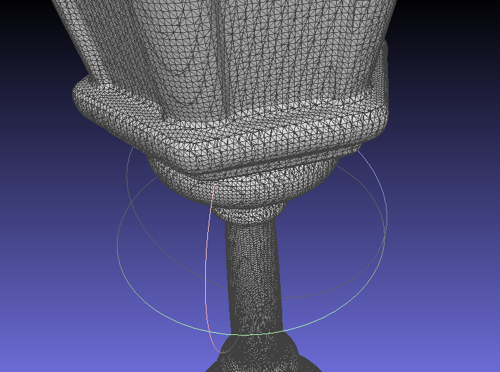
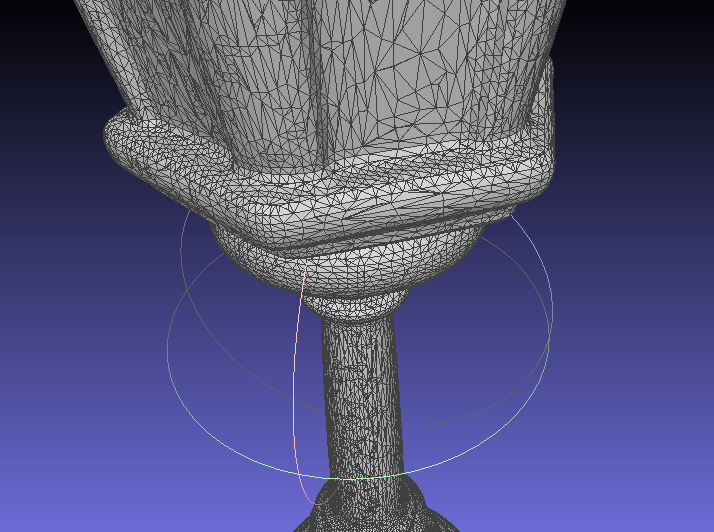
Figure 5: (a) Original triangular mesh; (b) Triangular mesh after edge collapse with Morton sorting.
Results: Table 1 reports mean times and the mean of the five paired speedup ratios. Morton had the lowest simplification and combined times. Tipsify and Hilbert also significantly accelerated simplification, although their preprocessing costs were higher than Morton’s. Nevertheless, all three locality-aware layouts produced a significant improvement over the randomized baseline.
Table 1: Mean timing, simulated average cache miss ratio (ACMR), and paired percent reductions over five trials. ACMR is the average number of simulated vertex-cache misses per triangle. Combined time and reduction include ordering and simplification.
References: [1] Fernando Cacciola, Mael Rouxel-Labbé, and Baskın Şenbaşlar. “Triangulated Surface Mesh Simplification.” CGAL User Manual, CGAL 6.2. https://doc.cgal.org/latest/Surface_mesh_simplification/ Accessed August 26, 2026. [2] G. M. Morton. “A Computer Oriented Geodetic Data Base and a New Technique in File Sequencing.” IBM Ltd., Ottawa, Ontario, Canada, Technical Report, 1966. https://books.google.com/books?id=9FFdHAAACAAJ [3] Hans Sagan. Space-Filling Curves. Universitext. New York: Springer, 1994. https://doi.org/10.1007/978-1-4612-0871-6 [4] Pedro V. Sander, Diego Nehab, and Joshua Barczak. “Fast Triangle Reordering for Vertex Locality and Reduced Overdraw.” ACM Transactions on Graphics, vol. 26, no. 3, article 89, 2007. https://doi.org/10.1145/1276377.1276489 [5] Peter Lindstrom and Greg Turk. “Fast and Memory Efficient Polygonal Simplification.” In Proceedings of IEEE Visualization 1998, pp. 279–286, 1998. https://doi.org/10.5555/288216.288288
In the first session of the project, the mentors taught us something that reshaped how I communicate basically anything. They called it the “Funnel method” and what it means is that when you have been thinking about something for so long, it´s very easy to subconciously assume that the person to whom you explain that thing has been thinking about it with you and has enough context to understand everything you are saying, but this is almost never the case, and this is where the funnel method comes in.
It involves explaining something very broadly first, and slowly guiding your listener or reader (in this case), to the specific thing you wanted to communicate, kind of like how a funnel is shaped with a wide top and a very thin base.
Even though it may seem trivial at first glance, knowing it, is very different from actively practicing it.
Weeks later and I still find myself thinking about this analogy before explaining anything. Thank you Silvia Sellán and Ningna Wang for teaching me this.
I plan to put this method into practice in this blog post, and I´ll leave it to you, the reader, to decide how well I was able to distill what I wanted to communicate.
Why slices?
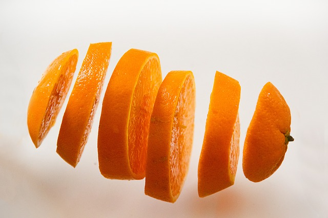
Yes I do mean the slices you are thinking of, the same slices you get when you cut an orange or bread.
Now think of an MRI machine or an Ultrasound scanner. In a way, they are both very sophisticated slicers. They do not physically cut an object apart, of course. Instead, they let us observe 2D cross-sections of something that exists in 3D Each image gives us only a thin view of the whole structure, much like cutting through a loaf of bread and looking at one slice at a time.
This gives us an interesting inverse problem: if we are given 2D slices, can we reconstruct the 3D object they came from?
Where could this be applied?/Why should you care?
In medicine, imagine if doctors can accurately visualize abnormalities such as tumors in 3D. This would help with treatment planning and even preparation for surgeries, through virtual surgery simulations. It can also help notice abnormalities that can´t be clearly captured by observing slices independently.
In archaeology, most artifacts are very delicate making accessing the inside components without destroying them very difficult, but if we can do 2D scans and reconstruct the 3D appearance we can solve this.
And many many other applications……
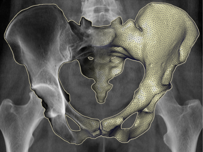
Figure 1. 3D reconstruction of pelvic anatomy from a 2D X-ray image. Source: Zuse Institute Berlin (ZIB), “3D Reconstruction of Anatomical Structures from 2D X-ray Images.
Our approach: Learning-based 3D Reconstruction
Simply: We use machine learning to train a model on 2D cross-section data and have it predict the original 3D shape
In detail:
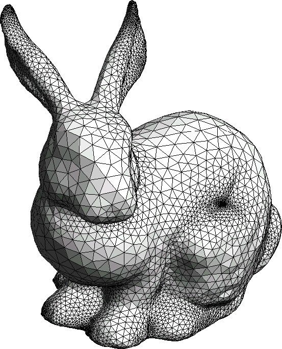
To begin we chose to build a pipeline that works for the “Stanford bunny” which is a widely recognized shape, and validate it with other shapes and cross sections after .
Figure 2. The Stanford Bunny
Data Preparation
Creating the cross-sections
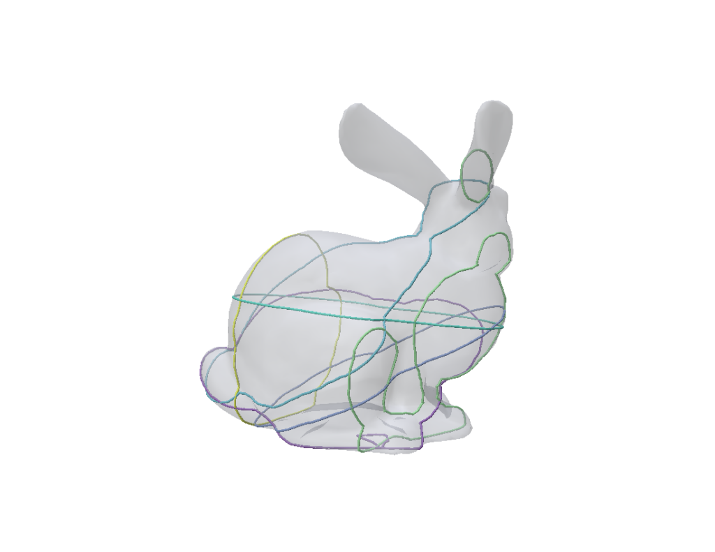
We first repair and normalize the bunny before cutting it with six virtual planes. Each plane intersects the surface and produces one or more 2D contour curves describing the object’s shape at that location.
Figure 3.The Stanford Bunny intersected by six virtual planes. Each colored curve represents an observed cross-section.
2. Next, we convert each contour into a 2D signed distance field, or SDF. A contour tells us where the boundary of the slice is, but an SDF gives us a little more information. For every point on the slicing plane, it tells us whether that point is inside or outside the contour and how far away from the contour it is.
For a point x and a contour C, the 2D signed distance field is defined as:
The equation looks more complicated than the idea behind it:
A negative value means the point is inside the cross-section.
Zero means the point lies directly on the contour.
A positive value means the point is outside the cross-section.
The size of the value tells us how far the point is from the contour.
A circle gives a simple example. For a circle with center c and radius r, the signed distance field is:
If a point is closer to the center than the radius, it lies inside the circle and gets a negative value. A point exactly one radius away lies on the boundary and gets zero, while anything farther away gets a positive value.
So instead of giving our model only the outline of each cross-section, we also give it information about the space around that outline.
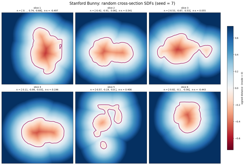
Figure 3. The six cross-sections represented as signed distance fields. The magenta lines are the observed contours; red represents the interior, blue represents the exterior, and white approaches zero distance.
Mapping the observations into 3D
3. We place the slice information into a 64 × 64 × 64 voxel grid, giving us 262,144 possible locations in 3D space.
For each voxel that lies on one of the observed slices, we store a few pieces of information: whether it was actually observed, its signed distance from the 2D contour, the direction of the slicing plane, and its 3D distance from the nearest observed contour.
Together, these give us six input channels:
one channel marking which voxels were observed,
one containing the 2D signed-distance values,
three describing the plane normal,
and one containing the distance to the nearest contour.
So the input to the model has the shape
The important part is how little of this grid we actually know. With only six slicing planes, just 24,973 out of 262,144 voxels contain observations, about 9.53% of the full volume.
That means the model sees less than 10% of the 3D space directly. Its job is to figure out what the object should look like in everything that remains.
Video 1: Sweeping through the 3D SDF grid reveals the Stanford Bunny at the zero level set. Video 2: The observed cross-sections retain 24,973 voxels 9.53% of the full grid shown around the ground-truth bunny.
Predicting the complete 3D shape
4. A 3D U-Net takes this sparse input and predicts a signed distance value for every voxel in the grid, including the many locations that were never observed by any of our slices.
We can write the model’s prediction as:
with
Here, fθ is our 3D U-Net and θ represents the parameters it learns during training.
Just like with the 2D SDF, the sign of the predicted value tells us where a point lies relative to the object:
The difficult part is that the model has only seen a small fraction of the grid through our slices. It therefore has to fill in what happens in the large spaces between them.
Training the reconstruction model and Preliminary results
During training, the U-Net parameters are adjusted to minimize a loss function. The loss determines which information the model is allowed to use and which geometric properties the reconstructed field should satisfy.
To compare the different training strategies fairly, we use the same six-channel input tensor, 3D U-Net architecture, random seed, optimizer and voxel resolution. We then change only the loss function or the constraint applied to the network’s output.
1. Supervised reconstruction
For our first training run, we make the problem easier for the model by giving it access to the complete ground-truth 3D signed distance field during training. In other words, for every voxel, we already know what the correct SDF value should be, and the model learns by comparing its prediction with that answer.
To measure how far the prediction is from the ground truth, we use a truncated L1 loss:
Symbols:
L sᴅꜰ is the supervised SDF loss.
Ω is the complete 3D voxel grid.
|Ω| is the number of voxels in the grid.
x is one voxel location.
φ̂₃D(x) is the predicted distance.
φ₃D(x) is the ground-truth distance.
τ is the truncation distance, set to 0.1.
clip(a, −τ, τ) restricts a value so that it cannot be smaller than −τ or larger than τ.
Σ means that the error is added across all voxels.
The idea behind truncation is simple. We care most about getting the region close to the object’s surface right. Very large distances far away from the bunny are less useful for reconstructing its actual shape, so we cap them at:
with:
This means that values smaller than -0.1 are treated as -0.1, while values larger than 0.1 are treated as 0.1.
The model therefore focuses more strongly on the region around the zero level set:
This is important because the zero level set is where the surface of the bunny lies.
This experiment gives us a useful reference point. Since the model can see the complete answer during training, we can first check whether our U-Net and input representation are capable of reconstructing the bunny at all. Later, we remove this ground-truth information and tackle the much harder problem of learning from the slices alone
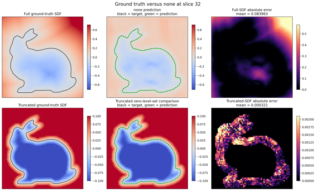
Figure 4. Supervised reconstruction at the central grid slice. Black shows the ground-truth zero level set, while green shows the predicted surface. The error maps show where the predicted and ground-truth SDFs differ.
2. Soft geometric constraint
The 2D cross-sections also give us a useful geometric rule. On an observed slicing plane, the predicted 3D distance should not be larger than the 2D distance measured on that slice:
Instead of forcing the model to satisfy this rule exactly, the soft constraint adds a penalty whenever the prediction breaks it:
Symbols:
Lbound is the soft-bound penalty.
Ωobs is the set of voxels belonging to the observed slices.
|Ωobs| is the number of observed voxels.
x is one voxel location.
φ̂3D(x) is the 3D signed distance predicted by the model at x.
φ2D(x) is the signed distance measured from the observed 2D slice at x.
|·| gives the magnitude of a signed distance, regardless of whether it is positive or negative.
max(0, ·) means that no penalty is added when the constraint is satisfied.
A positive penalty is added when the predicted distance exceeds the observed 2D distance.
So when:
the model receives no additional penalty.
But when:
the model is penalized based on how much it exceeds the bound.
We then combine this penalty with the supervised reconstruction loss:
Symbols:
Lsoft is the complete training loss for the soft method.
Lsᴅꜰ is the supervised reconstruction loss.
Lboundis the geometric-bound penalty.
The weight 2 controls how strongly bound violations are penalized.
Figure 5. Reconstruction using the soft slice bound. The model may violate the geometric bound, but each violation adds a penalty to the training loss.
3. Hard geometric constraint
The hard method does not merely penalize constraint violations. Instead, it changes the network output so that the geometric bound is guaranteed.
The final prediction is defined as:
Symbols:
is the raw U-Net prediction at voxel \mathbf{x}.
represents the U-Net’s learned parameters.
is the unsigned distance from \mathbf{x} to the nearest observed contour.
is the set of observed contour points.
restricts the raw prediction to a value between -1 and 1.
is the final constrained prediction.
The observed-distance field is calculated as:
This means that, for every voxel , we calculate the distance to the closest point on an observed contour.
Because always lies between -1 and 1, the prediction satisfies:
Therefore, the magnitude of the predicted signed distance cannot exceed the distance from that voxel to the nearest observed contour.
At an observed contour, equals zero. The prediction must therefore also equal zero:
The hard method still uses the complete ground-truth SDF during training. The difference is that contour consistency is guaranteed directly by the network output rather than encouraged through an additional penalty term.
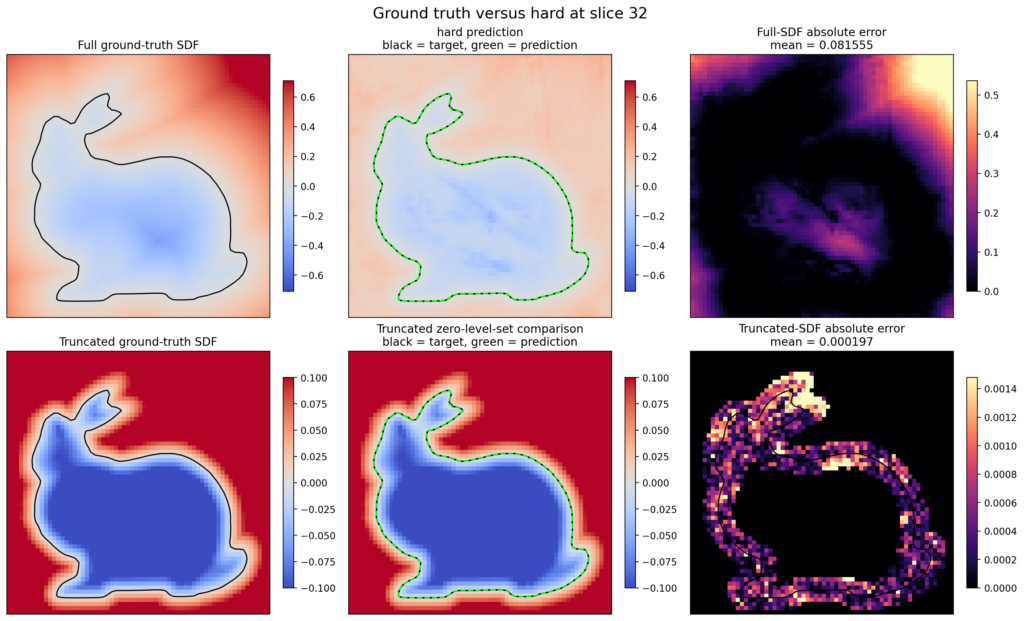
Figure 6. Reconstruction using the hard contour envelope. The black contour is the ground-truth surface and the green contour is the prediction.
4. Eikonal regularization
For a signed distance field to behave correctly, its gradient should have a magnitude close to one:
In other words, moving one unit in space should change the signed distance by roughly one unit. We encourage this property using the Eikonal loss:
Symbols:
is the Eikonal loss.
is the full voxel domain.
is the total number of voxels.
is the spatial gradient of the predicted field.
The squared term penalizes gradients whose magnitude differs from one.
The Eikonal term is added to the supervised SDF loss:
Symbols:
is the total training loss.
measures how closely the prediction matches the ground-truth SDF.
encourages the prediction to retain signed-distance-field behaviour.
determines how strongly the Eikonal term contributes to the total loss.
The main idea is simple: the supervised loss teaches the network what the SDF should look like, while the Eikonal term helps keep its spatial behaviour consistent with a true signed distance field.
Figure 7. Reconstruction with Eikonal regularization. This condition produces a field that behaves more closely like a valid signed distance field.
5. Slice-only reconstruction
The supervised experiments are useful for checking that our pipeline works, but they rely on something we would not normally have when reconstructing an unknown object: the complete 3D ground truth.
So we next try a harder setting inspired by CrossSDF. In this experiment, the model never sees the ground-truth 3D SDF during training. It has to learn only from the observed slices and from properties that we expect a valid signed distance field to satisfy.
The complete slice-only loss is:
Symbols:
is the complete slice-only loss.
encourages the reconstructed surface to pass through the contours that we actually observed.
penalizes predictions that disagree with the inside/outside information given by the slices.
encourages the prediction to behave like a valid signed distance field.
discourages the model from creating extra surfaces in places where we have no evidence that a surface should exist.
and control how strongly the two regularization terms contribute to the total loss.
On-contour loss
The first thing we want to guarantee is that the reconstructed surface agrees with the contours we actually observed.
We treat voxels within approximately one voxel width of an observed contour as on-contour points.
The on-contour loss is:
Symbols:
is the on-contour loss.
is the set of voxels treated as being on or very close to an observed contour.
is the number of voxels in that set.
represents one voxel location.
is the predicted 3D signed distance at .
is the signed distance given by the observed 2D slice at .
The absolute value measures the magnitude of the difference between the predicted and observed signed distances.
On the exact contour, the 2D signed distance is zero:
so this loss pushes the predicted 3D value toward zero as well:
Since zero represents the surface of an SDF, this encourages the reconstructed surface to pass through the contours that were actually observed.
Off-contour loss
Matching the contour itself is not enough. The slices also tell us which side of the contour is inside and which side is outside.
We therefore identify points where the predicted 3D SDF disagrees with the inside/outside information from the 2D slice.
The off-contour loss penalizes these disagreements:
Symbols:
is the off-contour loss.
is the set of voxels where the predicted and observed inside/outside information disagree.
is the number of voxels in that set.
represents one voxel location.
is the predicted 3D signed distance at .
is the signed distance observed on the 2D slice at .
Squaring the difference gives a larger penalty to larger disagreements between the predicted and observed signed distances.
Together, the on-contour and off-contour losses tell the model two things: where the observed surface is, and which side of that surface should be inside or outside.
Minimum-surface regularization
There is another problem when we remove the full 3D ground truth.
The model could satisfy the observed slices but still invent extra surfaces in the large regions between them. Since a surface occurs wherever the predicted SDF approaches zero, we want to discourage unnecessary near-zero values away from the observed contours.
We use the following minimum-surface regularizer:
Symbols:
is the minimum-surface regularizer.
is the region where this regularizer is evaluated.
is the number of voxels in that region.
represents one voxel location.
is the predicted 3D signed distance at
is the exponential function.
controls how strongly predicted values close to zero are penalized.
In our implementation:
When the predicted SDF is close to zero, the exponential term becomes large and adds a stronger penalty. As the prediction moves farther away from zero, the penalty becomes smaller.
This helps discourage the network from creating surfaces in regions where the slices provide no evidence that one should exist.
Most importantly, none of these slice-only loss terms use the complete ground-truth 3D SDF. The ground truth is kept aside and used only afterward to evaluate how close the reconstruction is to the real object.
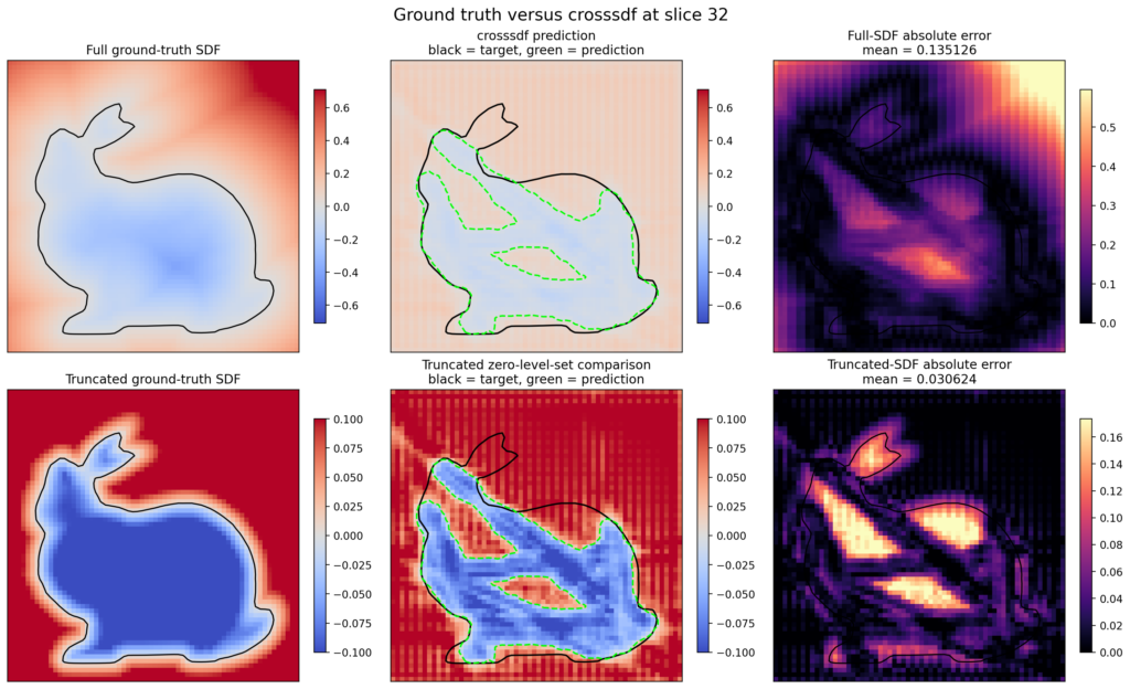
Figure 8. Initial slice-only reconstruction. The green predicted zero level set differs substantially from the black target contour, particularly around the ears and back
Evaluation metrics
Before comparing the reconstruction methods, we define three measurements that capture different aspects of geometric accuracy.
1. Intersection over Union
Intersection over Union, or IoU, measures the volumetric overlap between the predicted and ground-truth objects.
Let P represent the voxels predicted to be inside the object and G represent the voxels inside the ground-truth object.
Here, contains the voxels that are inside both shapes, while contains the voxels that are inside either shape.
An IoU of represents perfect overlap. An IoU of 0 means that the two interiors do not overlap. Therefore, higher IoU values are better.
2.Chamfer distance
Chamfer distance measures the average separation between the predicted and ground-truth surfaces.
Let A contain points sampled from the predicted surface and B contain points sampled from the ground-truth surface.
For each point on one surface, we find the nearest point on the other surface. These distances are then averaged in both directions.
A smaller Chamfer distance means that the two surfaces are closer on average. However, averaging can hide a small but severely incorrect region.
3. Hausdorff distance
Hausdorff distance measures the largest nearest-surface error.
Instead of averaging all surface distances, Hausdorff distance retains the largest error. It therefore measures the worst local failure in the reconstruction.
A lower Hausdorff distance means that even the least accurate part of the prediction remains close to the ground truth.
Why we use all three metrics
Each metric answers a different question:
IoU: How much of the predicted volume is correct?
Chamfer distance: How close are the surfaces on average?
Hausdorff distance: What is the largest local surface error?
A reconstruction can have a good Chamfer distance but a poor Hausdorff distance if most of its surface is accurate while one feature, such as an ear, is badly reconstructed.
In our results, Chamfer and Hausdorff distances are multiplied by 100 to make the values easier to read. This scaling does not change the comparison between methods.
We also report three diagnostic measurements:
Mean absolute error: the average absolute difference between predicted and ground-truth SDF values.
Surface MAE: the average SDF error near the ground-truth surface.
Eikonal error: how far the gradient magnitude of the predicted field deviates from one.
Lower values are better for all three diagnostic measurements.
Experimental setup
Our main experimental question is:
If the input and network remain fixed, how does changing the training objective affect reconstruction quality?
Every method uses the same Stanford Bunny, six cross-sections, six-channel input tensor and 3D U-Net architecture.
The input resolution is:
For the initial controlled comparison, we also keep the network initialization, optimizer, training duration and other hyperparameters fixed.
Voxel resolution: 64 × 64 × 64 Observed planes: 6 Training steps: 100,000 Base channels: 16 Learning rate: 5 × 10⁻⁴ Weight decay: 1 × 10⁻⁵ SDF truncation: 0.1 Random seed: 11 Optimizer: Adam
The supervised methods can compare their predictions with the complete ground-truth 3D signed distance field during training.
The slice-only CrossSDF method does not receive the complete target. It learns only from the observed cross-sections and general geometric properties of signed distance fields.
After training, marching cubes extracts the predicted zero level set as a triangle mesh. The ground-truth bunny is then used to calculate IoU, Chamfer distance and Hausdorff distance.
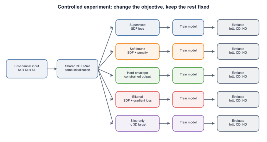
To make the comparison as controlled as possible, every condition receives the same input and uses the same 3D U-Net initialization.
We change only the training objective or the constraint applied to the output.
Figure 9. Controlled experimental design. Each condition receives the same six-channel input and uses the same 3D U-Net initialization. Only the training objective or output constraint changes. All reconstructions are evaluated using Intersection over Union, Chamfer distance and Hausdorff distance.
This controlled comparison covers the five original training conditions. The later CrossSDF refinement is treated as a separate follow-up experiment because it also changes the learning-rate schedule, contour regularization and number of training steps.
At this preliminary stage, each network is optimized and evaluated using the same Stanford Bunny. Therefore, these experiments test the reconstruction pipeline and effects of different losses; they do not yet demonstrate generalization to unseen objects.
Experiments and results
The previous sections introduced the loss functions we used in training, the metrics we used for evaluation, and the settings we had when doing the experiments.
Here, we focus on the results we got from each experiment, what we learned, and how this informed the next iteration of expermiments.
Experiment 1: Comparing the training objectives
We first compared supervised reconstruction, soft constraints, hard constraints, Eikonal regularization, and slice-only CrossSDF.
Method
Complete 3D target used during training?
IoU ↑
Chamfer ×100 ↓
Hausdorff ×100 ↓
Supervised reconstruction
Yes
0.9930
1.266
4.694
Soft constraint
Yes
0.9904
1.264
4.335
Hard constraint
Yes
0.9959
1.250
4.323
Supervised + Eikonal
Yes
0.9957
1.267
4.328
Initial slice-only CrossSDF
No
0.5862
8.891
62.263
All four supervised methods achieved IoU values above 0.99. This confirms that the input representation and 3D U-Net can reproduce the bunny when the complete target is available during training.
The hard-constrained supervised method produced the highest IoU and the lowest Chamfer and Hausdorff distances. The Eikonal method achieved similar surface accuracy while producing a field that behaved more closely like a valid signed distance field.
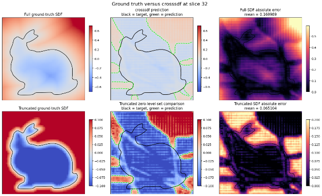
The slice-only CrossSDF result was substantially less accurate. It achieved an IoU of 0.5862, a Chamfer distance of 8.891 and a Hausdorff distance of 62.263.
Figure 10. Ground-truth and initial CrossSDF fields at the central grid slice. The black curve represents the target surface and the green curve represents the predicted zero level set. Brighter areas in the error map indicate larger disagreement.
What we learned?
The supervised experiments show that the network has enough capacity to represent the bunny. The main difficulty is therefore not simply that the architecture is too small. The difficulty comes from reconstructing unobserved geometry without a complete 3D target.
Only a small portion of the volume is observed by the six slicing planes. Many different 3D surfaces could pass through the same contours, allowing the prediction to agree with the observed slices while remaining incorrect between them.
Based on this result, we considered four possible explanations:
The unconstrained network could create unsupported geometry.
Combining overlapping slicing planes could discard information.
Six cross-sections might not contain enough geometric information.
The optimization schedule might not be appropriate for CrossSDF.
We investigated these possibilities through several follow-up experiments.
Experiment 2: Adding a hard global bound
The initial slice-only CrossSDF method used the network’s raw output directly.
This allowed the predicted distance field to take unsupported values away from the observed contours.
We therefore added the hard contour envelope defined earlier.
Here, Uobs(X) is the distance from a voxel to the nearest observed contour.
Because the hyperbolic tangent remains between and the resulting field satisfies the following bound.
At an observed contour, Uobs(X) = . The predicted 3D SDF must therefore also equal zero at that location.
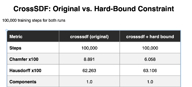
Both CrossSDF versions were trained for 100,000 steps.
Figure 11. Quantitative comparison between the original CrossSDF reconstruction and CrossSDF with the hard contour-distance bound.
The hard bound reduced the Chamfer distance from 8.891 to 6.058. The predicted surface therefore became closer to the target on average.
However, the Hausdorff distance increased slightly from 62.263 to 63.106.
What we learned?
The hard bound improved most of the reconstructed surface, but it did not correct the worst local failure.
This result demonstrates why Chamfer and Hausdorff distance must be considered together. Chamfer reports that average surface accuracy improved, while Hausdorff reveals that at least one highly inaccurate region remained.
Experiment 3: Multiplane supervision
Where slicing planes overlap, combining their observations into one voxel value may discard information.
We therefore calculated the on-contour and off-contour losses separately for each of the six planes and averaged the results.
The multiplane loss can be summarized as follows.
Here:
K is the number of slicing planes.
ℒon(k) is the on-contour loss for plane k.
ℒoff(k) is the off-contour loss for plane k.
In our experiment:
K=6
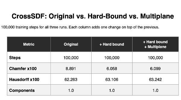
The hard envelope remained active, and all versions were trained for 100,000 steps.
Figure 12. Quantitative comparison between the original CrossSDF reconstruction, CrossSDF with the hard contour-distance bound, and a variation that adds multiplane supervision.
What we learned ?
Preserving supervision from each slicing plane did not improve this particular reconstruction by itself.
This does not prove that overlapping-plane information is unimportant. Instead, it shows that information loss at plane intersections was not the only cause of the reconstruction error. Sparse observations and optimization behaviour remained important.
Experiment 4: Refining the optimization process
Longer training with a fixed learning rate did not consistently improve the slice-only reconstruction.
For the final refinement, we combined:
The hard contour envelope.
Separate losses for all six slicing planes.
Minimum-surface regularization outside the observed contour band.
Cosine learning-rate decay.
Target-free checkpoint selection.
The learning rate decreased as follows.
The refined method improved every reported metric:
Metric
Initial CrossSDF
Refined CrossSDF
Mean absolute error
0.2496
0.2173
Surface MAE
0.0528
0.0488
IoU
0.5862
0.7743
Eikonal error
0.1195
0.0932
Chamfer ×100
8.891
5.159
Hausdorff ×100
62.263
54.388
IoU increased from 0.5862 to 0.7743, showing substantially better volumetric overlap.
Chamfer distance decreased from 8.891 to 5.159, indicating better average surface accuracy. Hausdorff distance also decreased from 62.263 to 54.388, although it remained much larger than the supervised results.
What we learned?
The optimization strategy had a substantial effect on slice-only reconstruction. The refined model achieved better results using fewer training steps.
However, several components were changed simultaneously. We cannot yet determine whether the improvement came mainly from the learning-rate schedule, hard envelope, multiplane losses or contour-aware regularization.
The refined experiment also used a different number of training steps. It should therefore be presented as a follow-up refinement rather than as part of the strictly controlled 100,000-step comparison.
Experiment 5: Locating the remaining surface error
Although the refined method improved all the numerical metrics, its Hausdorff distance remained relatively high.
We therefore visualized the distance between the predicted and ground-truth surfaces to locate the remaining error.
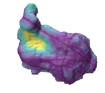
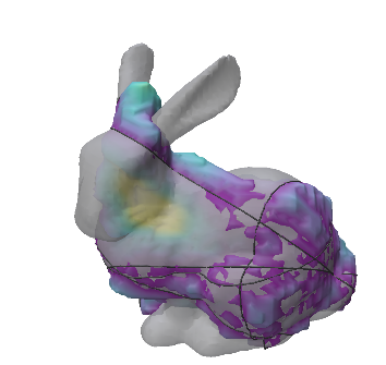
Figure 13.Surface-error visualization of the refined slice-only reconstruction. The shape shown is the reconstructed output. The black curves indicate the observed cross-sections, while the yellow patch highlights the region with the largest reconstruction error.Figure 13.1 shows the ground truth (in grey) merged with the networks output to show you what the network couldn´t predict (also in grey)
What we learned?
The error was concentrated in particular regions rather than distributed evenly across the entire bunny.
Most of the predicted surface was relatively close to the target, explaining the improvement in Chamfer distance. However, a smaller region remained far from the correct surface, keeping the Hausdorff distance high.
The visible gray geometry represents parts of the ground-truth bunny that the prediction did not recover. This demonstrates how a reconstruction can appear approximately bunny-shaped while still missing important local features.
Experiment 6: How does the number of cross-sections affect reconstruction?
Our main experiments used six cross-sections. In Experiment 6, we investigated how the reconstruction changes when the model receives eight and sixteen slicing planes.
Increasing the number of slices provides more direct information about the object and reduces the size of the unobserved regions between the planes. However, the result still depends on whether those planes intersect important local features.
These experiments used different training settings from the main 100,000-step comparison, so we treat them as exploratory results.
Reconstruction using eight slices
With eight slicing planes, the observations capture parts of the bunny’s body, head and lower structure. However, several important local features remain unobserved.
Figure 14. Ground-truth bunny and reconstruction using eight slicing planes. Black curves show the observed cross-sections. The sparse observations capture the approximate body but fail to preserve some local features.
The prediction has the approximate size and orientation of the bunny, but its geometry remains irregular. One ear is missing from the main surface and appears as a disconnected component. The lower body and front of the bunny also contain unsupported extensions.
Reconstruction using sixteen slices
We then increased the input to sixteen slicing planes. The additional planes provide denser coverage of the head, ears, body and lower structure.
Figure 15. Ground-truth bunny and reconstruction using sixteen slicing planes. The additional cross-sections provide more information about the global structure and local features.
The sixteen-slice prediction is more recognizable as a bunny. Both ears are connected to the main surface, and the overall head and body structure are more complete.
However, the reconstructed surface remains rough and distorted. Additional slices improve the available evidence, but they do not completely solve the reconstruction problem.
What we learned from Experiment 6?
Increasing the number of slices helps the model recover features that were missing from the sparser input. More slices also reduce the distance between observed regions.
However, matching more contours does not guarantee that the surface between them will be correct. The result still depends on where the planes are positioned and which features they intersect.
The experiment therefore shows that both the number and placement of cross-sections affect reconstruction quality.
Experiment 7: Can we provide too many cross-sections?
In Experiment 7, we tested much denser input containing up to fifty slicing planes.
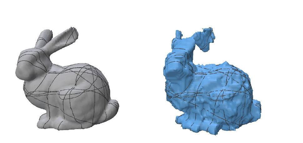
The reconstruction is considerably more recognizable than the results obtained from sparse inputs. The ears, body, legs and tail are all represented in the predicted mesh. However, this result must be interpreted carefully. With 50 slicing planes, much of the object has already been observed, so the network has fewer large regions of missing geometry to infer.
What we learned from Experiment 7?
More cross-sections do not automatically create a better scientific experiment.
Although 50 slices produce a more recognizable reconstruction, they also weaken the shape-completion challenge because much of the target geometry is already visible in the input.
The goal is therefore to identify the smallest and most informative collection of cross-sections from which the model can reliably reconstruct the unobserved 3D geometry.
Experiment 8: Does the way we select the planes matter?
The previous experiments showed that adding more cross-sections can improve reconstruction. However, the number of planes is not the only important factor. Their positions and orientations determine which parts of the object are actually observed.
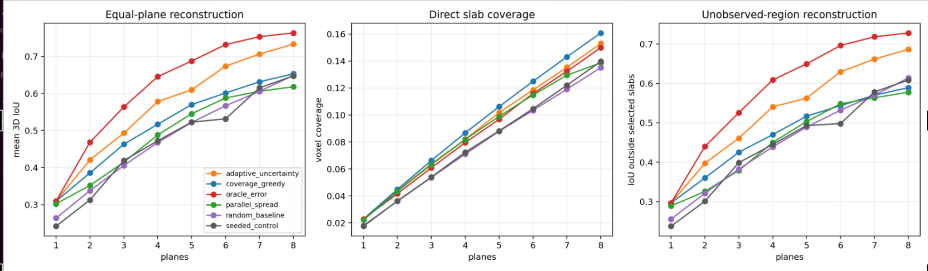
In Experiment 8, we compared six ways of selecting the slicing planes:
Random baseline: selects each plane randomly.
Parallel spread: places parallel planes at different positions across the object.
Coverage greedy: selects the plane that covers the largest amount of previously unobserved space.
Adaptive uncertainty: selects a plane through a region where the current reconstruction is most uncertain.
Seeded control: uses a fixed and reproducible collection of planes for comparison.
Oracle error: selects a plane using knowledge of the true reconstruction error. This information would not be available for an unknown object, so the oracle represents an ideal upper bound rather than a practical method.
Each method was evaluated using the same number of planes.
Figure 16. Comparison of six plane-selection strategies. Left: overall 3D IoU. Middle: the portion of the volume directly covered by the slices. Right: IoU in regions that were not directly observed.
The left graph shows that reconstruction generally improves as more planes are added. Oracle-error sampling produces the highest IoU because it always targets regions where the reconstruction is known to be wrong.
Among the practical strategies, adaptive uncertainty performs best. Instead of simply covering more space, it asks where a new observation would be most useful.
The middle graph shows that coverage-greedy sampling directly observes the largest portion of the volume. However, it does not produce the best reconstruction. A plane can cover many new voxels without intersecting an important feature.
The right graph measures accuracy outside the selected slices. Adaptive uncertainty performs well here, showing that it helps the model reconstruct geometry that was never directly observed.
What we learned?
Plane placement matters as much as plane count. Selecting planes only to maximize coverage is not enough. It is more useful to place them through uncertain or geometrically important regions.
These results suggest an adaptive workflow: begin with a few slices, reconstruct the object, identify where the prediction is uncertain and then request a new slice through that region. This could produce an accurate reconstruction using fewer, but more informative, observations.
Beyond the Bunny
Most of our experiments focused on the Stanford Bunny. We also tested the reconstruction process on a more complex spider model containing several thin, closely spaced parts.
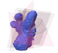
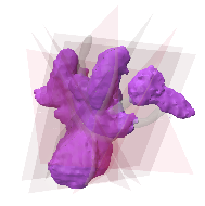
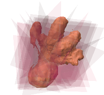
We reconstructed the spider using different numbers of cross-sections, represented by K.
K = 4
K= 8K=16
K=32
With only four or eight slices, the model captures the approximate volume but struggles to separate the individual parts. As more slices are added, the structure becomes clearer and more connected.
What we learned?
The spider is harder to reconstruct than the bunny because its thin parts can easily fall between the slicing planes. This example supports our earlier finding that complex local features require either more observations or more carefully selected planes.
It also shows why future evaluation should include several kinds of objects rather than relying only on the Stanford Bunny.
Overall findings
Our experiments show that reconstructing a complete 3D object from sparse 2D cross-sections is possible, but the quality depends on both the training method and the information contained in the slices.
When we gave the network access to the complete 3D target, all the supervised methods reconstructed the bunny very accurately, with IoU values above 0.99. This reassured us that the U-Net and voxel representation were working as intended.
The real challenge appeared when we removed the complete 3D target. The initial slice-only CrossSDF model reached an IoU of only 0.586. It could follow some of the observed contours, but it struggled to decide what the bunny should look like in the large spaces between them.
Adding the hard contour constraint helped the prediction stay closer to the observed geometry. However, it did not fix the worst local errors. Multiplane supervision also made sense in theory, but it was not enough to solve the problem on its own.
Our refined CrossSDF experiment produced the clearest improvement. By combining the hard constraint, multiplane losses, contour-aware regularization and a decaying learning rate, we increased IoU from 0.586 to 0.774. The bunny became more recognizable, although some important parts were still missing or incorrectly shaped.
The slice-count experiments also taught us that more data is helpful, but only up to a point. Eight slices missed important features, while sixteen gave the model a much clearer picture of the bunny. With 50 slices, however, so much of the object was already visible that the network had much less geometry left to infer.
Finally, we learned that where we place the slices matters just as much as how many we use. Simply choosing planes that cover the largest amount of space did not give the best results. Selecting planes through uncertain regions was more useful because those slices provided information the model actually needed.
Overall, our experiments suggest that a successful system should not rely on a fixed set of random cross-sections. A better approach would be to begin with a few slices, make an initial reconstruction, identify where the model is uncertain and then request new slices through those regions.
In other words, the most useful next slice is not necessarily the one that covers the most space. It is the one that answers the model’s biggest remaining question.
Future directions
Next, we want to test the method on more shapes to see whether it works beyond the bunny.
We also want the model to choose new slices through areas where it is most uncertain. Finally, we plan to test higher resolutions, noisy data, and real MRI or CT scans.
Acknowledgements
This project would not have been possible without the guidance and support of our mentors Silvia Sellán and Ningna Wang, and our volunteer: Vivien van Veldhuizen. Their feedback helped us implement the project and turn our ideas into clear experiments.
I am very grateful to the other SGI fellows on the project team: Shannon Cudworth, Gokul Adithya Suresh, Zane Beeai, and Yushi Huang, for the discussions, coding, testing, and visualizations that brought the project together. Thank you to everyone in the SGI community who shared their time, knowledge, and encouragement throughout the project.
Fluid motion in computer graphics is typically modeled by the incompressible Navier-Stokes equations:
where is the velocity of the fluid, density, pressure, body force and kinematic viscosity. The first equation (momentum) is Newton’s second law applied to fluid elements, and the second one constrains the flow to be volume-preserving.
An important concept is the material derivative, which measures the rate of change of a quantity following a fluid parcel (Lagrangian) rather than at a fixed point in space (Eulerian).
This allows us to write the momentum equation compactly as
and defines advection s.t. means the quantity is carried by the flow without changing.
Vorticity
Vorticity is defined as the curl of velocity , and measures the local rate of rotation of the fluid. For inviscid flow with no body force, taking the curl of the momentum equation gives the vorticity transport equation
where the right-hand side is the vortex-stretching term (as shown in Section 2.1, this term vanishes identically in the 2D setting used throughout this report, so vorticity there is materially conserved exactly, ); it is simply carried by the flow. This makes vorticity important for simulating turbulent and swirl-dominated phenomena, since instead of solving for pressure and velocity everywhere, one only tracks regions where vorticity is concentrated.
The key problem is recovering the velocity field given a vorticity field. In 3D, this is posed as a least-squares problem, i.e. find minimizing
solved via calculus of variations, yielding the Poisson problem , whose solution is the Biot-Savart law:
Deriving the 2D analogue
Jupiter’s bands and jet streams are a 2D phenomenon (a thin shell on the planet’s surface), so we re-derive the above for a 2D velocity field , where vorticity reduces to a scalar:
In this 2D setting points purely out of the plane while is purely in-plane, so the vortex-stretching term from Section 2 vanishes identically — not as an extra assumption, but automatically, because there is no out-of-plane direction left for vorticity to be stretched or tilted into. The vorticity transport equation therefore simplifies exactly to in 2D, which is what we use throughout.
As in 3D, we seek minimizing
Perturbing and using linearity of , the stationarity condition gives, with ,
Unlike 3D, maps a vector field to a scalar, so its adjoint maps a scalar back to a vector. Integrating by parts term by term (boundary terms vanish as fields decay at infinity),
so that, since this must vanish for all ,
The same vector identity used in 3D,
restricted to 2D becomes . With the constraint , we obtain a Poisson problem:
The 2D fundamental solution of the Laplacian is
satisfying , verified by the divergence theorem on the unit circle:
The solution to the Poisson problem, via convolution with :
Integrating by parts once again (moving off onto ) gives the 2D Biot-Savart law in the form:
Discretizing as a sum of Dirac deltas collapses the integral to a sum:
Since inviscid vorticity is materially conserved, each point vortex simply moves with the velocity induced by all other vortices at its own location (the self-term is excluded), giving the point vortex dynamics equation:
This is the equation we implemented and verified on various examples (e.g. leapfrogging etc.) before extending it to the sphere.
Implementation and Validation in the Plane
The point vortex dynamics equation above was implemented in Houdini using a custom SOP Solver: each timestep, a VEX wrangle reads the previous frame’s point cloud (position and circulation per point), evaluates the Biot–Savart sum, and advances each point’s position. Before trusting this on any nontrivial configuration, it was validated against two exactly-solvable two-vortex cases: equal circulations , where both vortices orbit a common, stationary centroid on a circular path, and opposite circulations , where the pair instead translates together in a straight line at constant speed. Both matched their analytic period/speed formulas.
As a further, qualitative check, a classical four-vortex leapfrogging configuration (two counter-rotating pairs, arranged so the trailing pair periodically overtakes the leading pair) was simulated and reproduced the expected periodic behavior.
Trajectories of the four-vortex leapfrogging configuration at three points in the cycle (frames 20, 80, 140). Each mark traces the recent path of one vortex; the pairs periodically exchange places as they orbit and overtake one another.
A Vortex-Ring Model of Kelvin–Helmholtz Instability
To move from the plane to Jupiter’s spherical atmosphere, the point vortex equation was extended to the unit sphere by replacing the planar kernel with the spherical Biot–Savart law and integrating positions via the exponential map, , so that points remain exactly on the sphere regardless of step size. Because has no boundary, the total vorticity must also integrate to zero, — a constraint with no analogue in the plane, enforced here by construction (equal numbers of positive and negative vortices, or an explicit normalization step subtracting the mean circulation from every point).
On this spherical setup, a shear layer was modeled as a vortex sheet: a ring of point vortices along a line of latitude, one sign on each side of the interface, with a small sinusoidal perturbation added to seed the instability. With no additional forcing, mutual induction alone causes the shear layer to roll up into a periodic array of vortices, as expected from classical vortex-sheet theory.
A single vortex-sheet interface at three stages: the initial perturbed line (frame 50), partial roll-up into discrete billows (frame 250), and a more developed, mixed state (frame 450).
This was then generalized to several alternating-sign rings restricted to a narrower latitude band, approximating Jupiter’s alternating belt/zone structure. Passive marker particles (zero circulation, contributing nothing to the velocity field but advected by it) were added and colored with a Jupiter-like palette for visualization.
Multi-band configuration (M=3) at frames 20, 250, and 500. Marker particles, seeded uniformly, are progressively advected and mixed along the band-induced shear flow.
Modeling the Coriolis Effect
To incorporate planetary rotation, the momentum equation was written in a frame rotating with angular velocity . Taking the curl and combining terms gives the vorticity equation with a rotational source,
in place of the inviscid used above. This was implemented by updating each vortex’s circulation every step, , so that circulation is no longer materially conserved. This is a first, direct discretization of the effect; a more careful treatment (in particular, its interaction with the constraint over long integration times) is left for future work.
Discussion and Limitations
The point-vortex approach reproduces known analytic solutions in the plane, the classical leapfrogging trajectory, and qualitatively correct Kelvin–Helmholtz roll-up on the sphere, both for a single interface and for a multi-band configuration resembling Jupiter’s belts and zones. The Coriolis implementation here is a direct, unrefined discretization rather than a fully validated one, and the multi-band results are qualitative: parameters such as band spacing, perturbation amplitude, and desingularization radius were chosen for a visually clear roll-up rather than calibrated against a specific analytic growth rate or against Jupiter’s actual physical parameters. Extending the integrator beyond forward Euler, and validating the Coriolis term against a known conserved quantity, are the natural next steps.
My goal for this project was to implement visualization methods that help artists gauge the accuracy of skin weight transfer methods, which takes the skin weights from an already rigged mesh, and assigns the correct weights to the target mesh. I compared two different weight transfer methods. First, Maya’s built-in copySkinWeights: which takes a vertex on the unrigged mesh, finds the closest point on the source mesh, and interpolates the weights at that point to determine the weights at the vertex. Next, a method developed by EpicGames, which copies the weights from the source mesh that have a high-confidence correspondence. For the remaining vertices, it computes the weights by interpolating from the transferred high-confidence weights.
To begin, I downloaded a character with an animation from Mixamo and imported it into Maya. In my first pass comparison, I unbound the shirt from the character, and then rebound it using Maya’s copySkinWeights and EpicGames’ Weight Inpaint method. Below is a playblast of each character. Notice that with the copySkinWeights there is a jagged concave area in the upper back region, while with the Weight Inpaint method, that area is smooth.
Now, I wanted to develop a method to visually compare the two algorithms. I created a heatmap using the error formula.
Expanding on the previous idea, I wanted to develop a dynamic heat map that shows the areas with the highest deformation error over the entire animation. I created a node that took the display/method mesh and reference mesh as inputs, and then took the 3D vertex position of each of the meshes. To calculate the deformation error, I calculated the Euclidean distance between the 3D vertex positions of the method I was evaluating and the 3D vertex position of the original mesh. This is calculated with:
where i represents the ith vertex of the matrix, is the 3D position of vertex i on the method mesh at frame t, is the 3D position of vertex i on the original method at frame t.
To construct the heat map, we normalize and clamp with:
where c is the maximum deformation distance.
We then mapped the errors to colors and wrote all vertex colors to the output mesh with setVertexColors(). We then have our finished output mesh with our desired heatmap. As the animation changes, the input meshes will change, causing the heatmap to update with each frame. This was packaged into a UI for easier use.
Here is the heat map applied to a shirt that was rigged using Maya’s copySkinWeights:
Here is the heat map applied to a shirt that was rigged using EpicGames Inpaint method:
TextDeformer: How can words shape the (virtual) world
Researched by: José Pablo Soto Sánchez
Introduction
Imagine handing a sculptor a block of clay and, instead of tools, just a sentence: “make this a giraffe.” No reference photos, no measurements, just words, and the expectation that the clay reshapes itself to match. That’s roughly what TextDeformer (Gao et al., SIGGRAPH 2023) does to a 3D mesh: given a source shape and a target text prompt, it deforms the geometry until a frozen vision-language model agrees that the render looks like the prompt.
What makes this interesting isn’t just the result it’s used purely as a differentiable critic. The actual “learning” happens directly on the geometry: a set of per-triangle Jacobian matrices gets optimized by gradient descent, the same way you’d optimize the weights of a network, except here the “weights” are literally how each triangle is allowed to stretch and rotate.
This post walks through reproducing the official TextDeformer codebase end-to-end on consumer hardware, the math that makes text-to-geometry gradients possible at all, and the specific things that broke along the way and how they got fixed.
Background
A few terms are worth pinning down before the method section, since the pipeline sits at the intersection of graphics and vision-language modeling:
Term
Plain-language definition
CLIP
A frozen, pretrained model that embeds images and text into the same vector space, so cosine similarity between an image embedding and a text embedding measures “how well does this image match this caption.”
Differentiable rendering
Turning a 3D mesh + camera into a 2D image using operations (rasterization, shading) that support backpropagation, so pixel-level loss can flow gradients back to vertex positions.
Jacobian (per-triangle)
A 3×3 matrix describing how a single triangle is locally stretched/rotated relative to its original shape. TextDeformer optimizes one of these per face, directly.
Poisson mesh reconstruction
Given a target Jacobian per triangle, solving a linear system to recover the vertex positions whose actual local deformation best matches those targets, in a least-squares sense.
Cotangent Laplacian
A sparse matrix built from mesh geometry that encodes how each vertex relates to its neighbors; it’s the operator at the center of the Poisson solve.
ViT patch
A Vision Transformer splits an image into fixed-size square tiles (“patches”) and treats each one like a token — patch size determines how fine-grained the model’s spatial resolution is.
Method
CLIP-guided losses
The core signal is cosine similarity between a rendered image’s CLIP embedding and the target text’s CLIP embedding:
But optimizing this alone tends to drift toward whatever image maximizes similarity to the prompt, not necessarily a smooth deformation of the source shape. TextDeformer adds a delta-CLIP term that instead matches the change in image embedding against the *change* in text embedding, relative to a fixed base render/prompt (e.g. “a cow”):
This directional formulation (used in prior CLIP-guided editing work) keeps the deformation anchored to the source identity instead of collapsing onto an unrelated “giraffe-like” blob.
Per-triangle Jacobians and the Poisson solve
This is the part that replaces a neural decoder entirely. Given the mesh’s gradient operator (one 3×3 block per face) and a diagonal mass matrix of face areas, the cotangent Laplacian is built as:
has a one-dimensional null space (constant functions), so the implementation drops the first row/column to pin a single vertex before it’s usable for Cholesky factorization. To go from optimized per-face Jacobians back to vertex positions , the code solves the normal equations of a least-squares problem — find the whose actual gradient is as close as possible to the target Jacobians , weighted by face area:
That linear system is factorized once per mesh with a sparse Cholesky solver (`cholespy`, GPU-resident) and re-solved every optimization step as changes — cheap after the one-time factorization. A Jacobian regularization term, , keeps triangles from stretching into degenerate shapes.
Rendering and camera augmentation
Each step, a batch of random cameras (elevation drawn from a Beta distribution, azimuth uniform over 360°, random distance/FOV/lighting/background) renders the current mesh via nvdiffrast‘s differentiable rasterizer. Randomizing viewpoint and lighting every step is what prevents the optimizer from exploiting a single “good” camera angle instead of actually deforming the geometry.
Patch-level consistency loss
A second, separate CLIP ViT is used only for its intermediate patch features (via forward hooks on each transformer block). For pairs of cameras within the same batch that are close in elevation/azimuth, the patches that project to the same 3D vertex are compared — encouraging the same surface point to look consistent from nearby viewpoints, which curbs the multi-view incoherence (“Janus-face”-style artifacts) common to CLIP-guided 3D optimization.
Implementation
Getting the reference implementation running at all.
The repo pins specific commits for nvdiffrast and installs igl unpinned via conda-forge. The unpinned igl immediately caused a break: igl.random_points_on_mesh in MeshProcessor.py expected a 2-tuple return (bary, face_idx), but the installed libigl build now returns a 3-tuple (B, FI, P). Fixed by unpacking a third, unused value — a reminder that “no version pin” in a 2023 paper repo means the API surface has already drifted.
Fighting the GPU context, not the geometry.
The next failure had nothing to do with the algorithm: dr.RasterizeGLContext() threw cudaGraphicsGLRegisterBuffer (CUDA error 304, cudaErrorOperatingSystem) on first render. [VERIFY: root cause inferred from the error code and hybrid-GPU laptop symptoms, not confirmed via driver-level logs] — the working hypothesis is that Windows was creating the OpenGL context on the integrated GPU while CUDA ran on the discrete GPU, breaking the CUDA↔GL interop nvdiffrast relies on. The pinned nvdiffrast commit doesn’t expose the pure-CUDA rasterizer (RasterizeCudaContext isn’t present in this build), so the fix was OS-level: explicitly forcing the Python process to the discrete GPU in Windows’ graphics settings, rather than a code change.
Finding the actual VRAM ceiling.
With rendering working, the default config (batch_size=25, train_res=512) ran out of memory on a 6 GB laptop GPU (RTX 4050) partway through the first step. The batch dimension and the render resolution both scale memory close to linearly, so both got reduced (batch_size=4, train_res=256) until a full 2,500-step run completed without OOM. This became the baseline configuration for every later experiment.
Swapping CLIP backbones without breaking assumptions baked into the code.
clip_model and consistency_clip_model are independently configurable, but the consistency-loss implementation (utilities/clip_spatial.py) hardcodes assumptions that only hold for the “Base” ViT variants: a for i in range(12) loop over transformer blocks (ViT-L/14 has 24), and an assertion that the patch stride evenly divides the patch size (ViT-L/14‘s 14px patch isn’t divisible by the default stride of 8, unlike 32px/16px). RN50 — a convolutional backbone — can’t be used for the consistency loss at all, since that code depends on ViT-style patch tokens that a ResNet simply doesn’t produce. ViT-B/32, ViT-B/16, and RN50 (as the primary loss only) were compared under an identical seed/mesh/prompt to keep the comparison controlled; ViT-B/32 was kept as the default going forward, primarily because it fit the VRAM budget without further code changes.
Debugging a mesh, not the code.
A custom tuna.obj mesh failed with CHOLMOD: not positive definite inside the Cholesky factorization. The Laplacian L is only positive-definite after pinning one null-space direction — which is correct for a single connected mesh, but insufficient if the mesh has multiple disconnected components (each contributes its own null direction). The tuna model’s eyes turned out to be separate, unwelded geometry. Diagnosing this required leaving the codebase entirely and going into Maya: using Mesh → Separate to count connected shells, Combine + Merge (vertex welding by distance) to attempt reattachment, and re-running Separate as the verification step (if it can no longer split the mesh, it’s genuinely one piece). Welding never fully closed the gap without visibly displacing the eyes during remeshing, so the pragmatic fix was deleting the eye geometry outright, producing tunaNoEyes.obj — a reminder that not every mesh bug is worth solving at the mesh level when the pipeline’s actual requirement (single connected component) can be satisfied more simply.
Stale caches and unattended runs.
MeshProcessor caches differential operators and Jacobian .npz files under <output_path>/tmp/ and silently reuses them if present — convenient for resuming, dangerous if the source mesh changes but the output path doesn’t: a later run against a re-exported (different vertex count) tuna.obj crashed in a sparse matrix multiply because the cached operators no longer matched. Once that class of bug was understood, a small driver script (run_batch.py) was written to chain multiple mesh/prompt runs sequentially — the single 6 GB GPU rules out any parallelism — each with a fresh output directory and its own log file, so a several-hour unattended batch could run overnight without one failed run silently corrupting the next.
Results
Five source→target pairs were run to completion on the final configuration (batch_size=4, train_res=256, ViT-B/32, single RTX 4050 Laptop GPU):
Source → Target
Steps
Wall-clock
cow → giraffe (spot.obj)
5,000
1h 14m
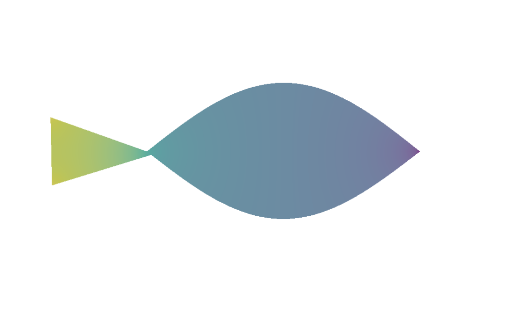
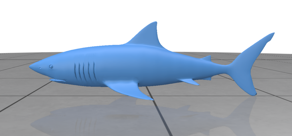
fish → shark
10,000
2h 37m
eiffel tower → rocket
10,000
3h 21m
tuna → shark (tunaNoEyes.obj, remeshed)
10,000
2h 33m
guitar → axe
600
9m 39s
Per-step cost stayed in a fairly narrow band (~0.89–1.2 s/step) across meshes of similar triangle count, and scaled with batch_size × train_res as expected from the rendering cost analysis above — the guitar → axe run at 600 steps was deliberately short (~10 minutes) as a fast-iteration sanity check rather than a converged result, and looks correspondingly less refined than the 10k-step runs.
Future Work
Validate mesh topology before the Poisson solve, not during it.
The tuna.obj failure surfaced as a Cholesky exception deep inside training, three layers of traceback away from the actual cause (disconnected components). A pre-flight check — counting connected components with igl and failing fast with a clear message before any GPU work starts — would turn a confusing runtime crash into an immediate, actionable one, and is a small, self-contained addition to MeshProcessor.py.
Generalize the consistency-loss encoder beyond the “Base” ViT assumption.
The hardcoded 12-layer loop and stride-divisibility requirement in clip_spatial.py make ViT-L/14 unusable for the consistency loss without a code change, and rule out testing community-trained checkpoints (e.g. LAION’s ViT-B-32 retrained on LAION-2B via open_clip) that share the same architecture but arrive through a different loading path than OpenAI’s clip package. Both are architecture-family limitations, not fundamental ones — worth fixing before running a broader backbone ablation.
We also explored a method for morphing one 3D shape into another target 3D shape. We worked with ShapeFlow, a neural network that learns to deform an existing 3D shape into another through a continuous flow field. Given latent space encodings of a source and target shape, the model outputs a velocity field describing how each point on the source should move to arrive at the target. Because the flow is continuous and (under the right conditions) bijective, the resulting deformation is guaranteed to be free of self-intersections, and can optionally preserve volume. Both of these properties can be desirable for artists working with meshes, which makes ShapeFlow attractive for toolification.
The Model
ShapeFlow’s creators frame the deformation of source shape into target shape as an advection process–the movement of a conserved property through fluid flow. Each point on the source is carried along a flow field over an interpolation parameter . Then, the points of the deformed source shape are described as:
Training seeks the mapping that minimizes the symmetric Chamfer distance between the deformed source and the target:
So the output of ShapeFlow is this flow field or mapping that describes how each point on the source shape should advect in order for the source to become the target shape. How are the inputs to ShapeFlow created? What do we feed to the model?
Recall, we said that the input to ShapeFlow is the pair of latent space encodings from the source and target shapes. For our implementation, we use an encoder that maps a mesh’s vertices to a latent space encoding using a single forward pass. The encoder is trained jointly with the deformer model, using the same Chamfer distance loss, so it learns to produce encodings that are useful for conditioning the flow field.
The Toolification
Our goal was to implement ShapeFlow as a Maya plug-in for artists’ use in stylization and retopology of one mesh to another. To increase usability, we added blendshapes between the source mesh and the deformed source mesh by extracting and exporting intermediate results along the deformation path (sampling at intermediate values of ). This way, an artist can scrub through the flow and select whichever stage best fits their needs.
Future Exploration & Improvement
While implementing ShapeFlow as a Maya tool for artists, we ran into some areas of exploration for the performance of the tool. With more time we would have done more experimenting and development to ensure the model’s capabilities are consistent and high-performing for our desired use cases. On the SGI timeline we ultimately decided to balance exploration and execution and forge ahead with building out the tool while noting areas for improvement:
Initialization Sensitivity: Since the initialization of the model weights are random, results can vary widely based on whether one initialization was “good” for the specific meshes being used.
Loss Function Limitations: One of the use cases we wanted to develop ShapeFlow for was to create intermediate expressions for a given face mesh with certain extreme expressions. However, when morphing between meshes that differ only in a small region–for example puckered lips vs. a neutral expression–the region may be too small to affect the Chamfer distance loss during optimization. Other loss functions are worth evaluating for these cases.
Pretraining: If there are certain use cases (classes of objects, faces) that ShapeFlow will be used for, it might be beneficial to do pretraining on those types of shapes. Currently, our tool trains the deformer model from scratch every time. (This is also why the initialization sensitivity affects the results so strongly.) As a result, the model either will take an extremely long time with an appropriate amount of training iterations, or be used after a lower number of training iterations with reduced fidelity.
We did some manual tuning to get workable results on our test meshes, but making this robust enough for an artist’s workflow requires additional experimentation, testing, and development.
Results
Below is a video demonstrating the Maya tool workflow. For the sake of time, in the video the model is only trained for 200 iterations (very low), which is one source of the poor or unfinished-looking output flow.
Below is an image showing how ShapeFlow can be used to produce a blend of two meshes. The ShapeFlow output (middle) is result of Toilet 1 (left) morphing into toilet 2 (right).
Project Members: Al Rahim Hossain, Stephanie Jung, Aleksa Milovanović, Reid Tang
Mentors: Otman Benchekroun, Ty Trusty
Introduction
Simulating deformable objects often requires optimizing over a large number of unknowns. For example, a 2D mesh with vertices has positional variables: an and coordinate for each vertex. A 3D mesh similarly has positional variables.
In a full order model, the deformed shape is represented by a vector containing all vertex positions. It is found by minimizing the total energy of the object:
where measures how much the object resists being deformed from its rest shape and represents external forces. The solution is the state with the lowest total energy, where the elastic response and external forces are balanced. However, this solution may be computationally expensive as it treats every vertex position as an independently moving variable.
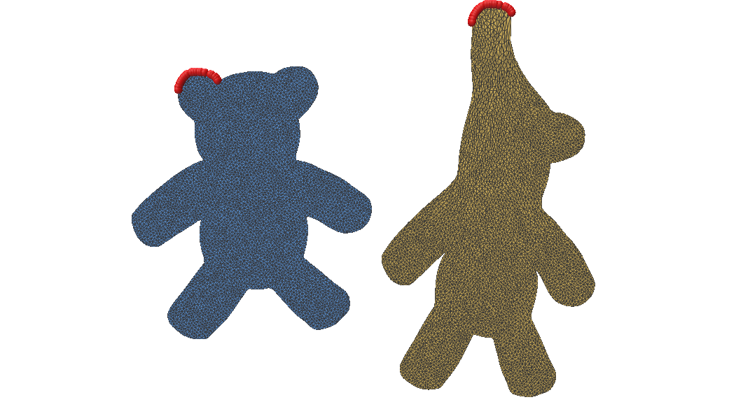
Figure 1: Comparison of the original 2D mesh (left) and its Neo-Hookean deformation (right) under gravity (), with fixed vertices highlighted in red. This represents the exact solution found using Newton’s method.
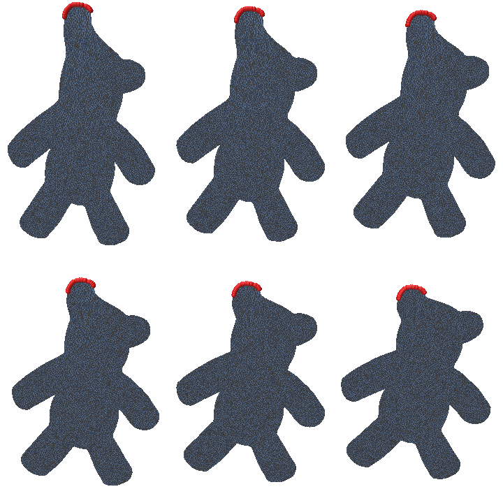
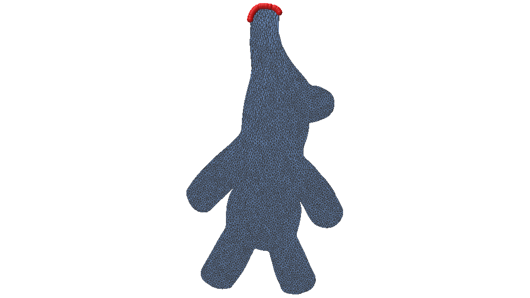
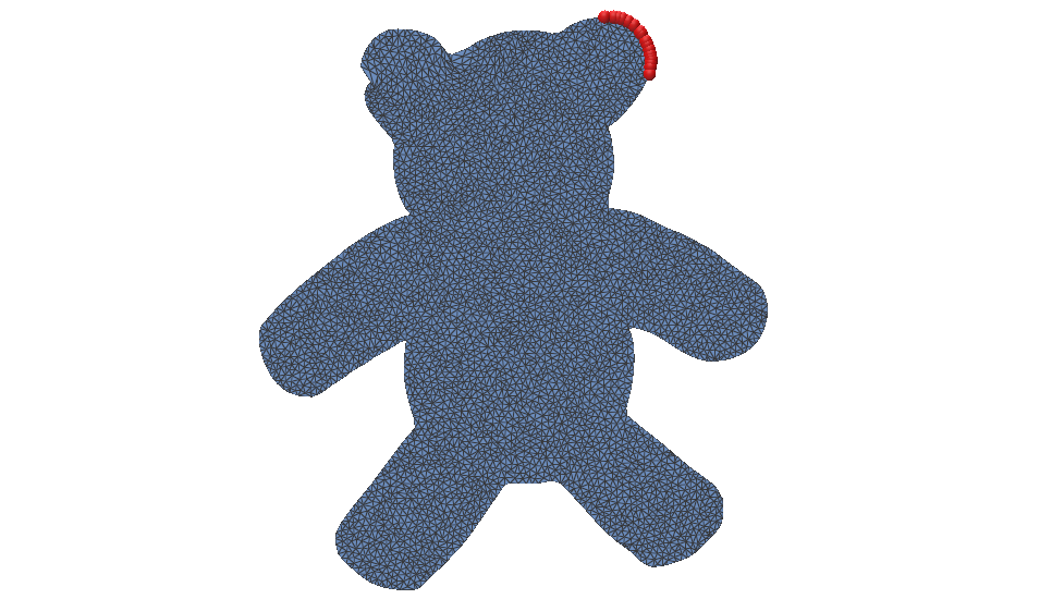
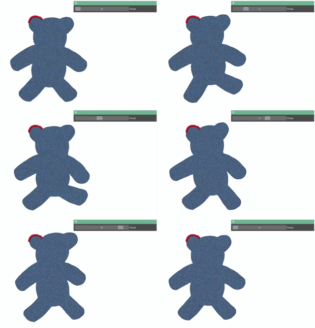
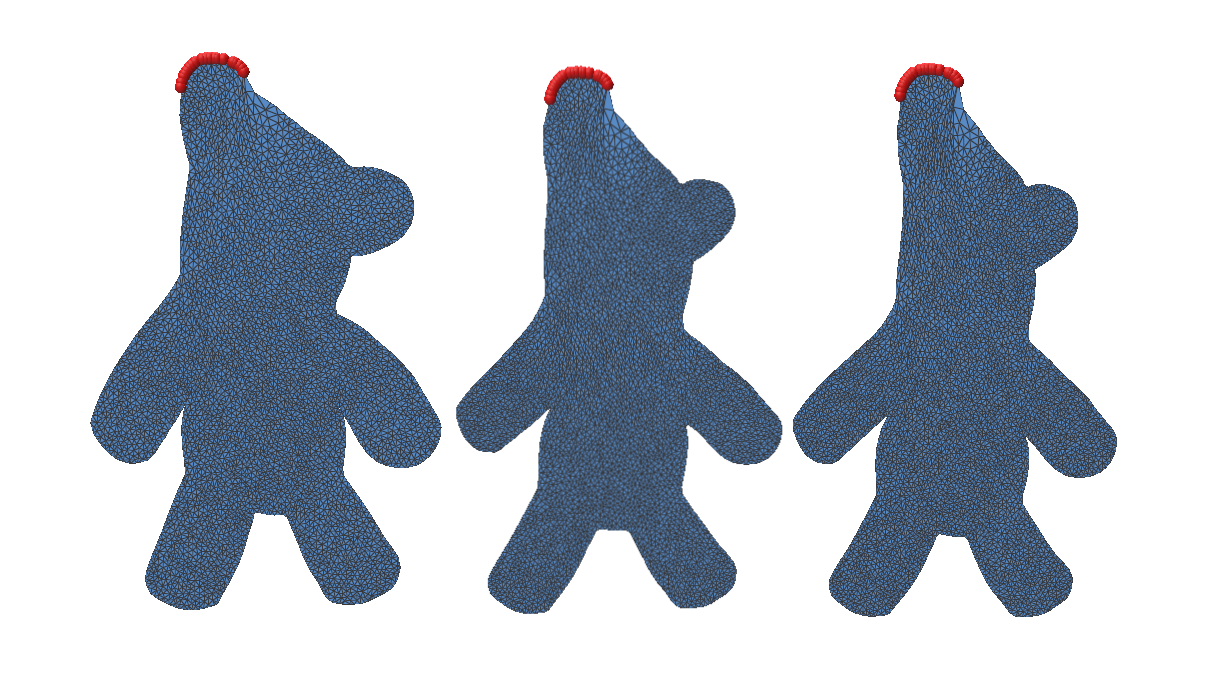
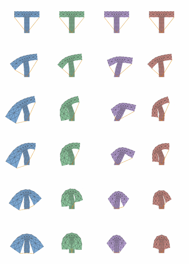
Reduced-Order Model
Reduced-order modelling reduces the size of this optimization by restricting the solution to a low-dimensional subspace. Instead of tracking every point independently, we choose a small set of meaningful deformation patterns. We then approximate the full configuration as where is the rest state of the object, the columns of matrix represent the selected deformation patterns, and vector contains their corresponding coefficients [1]. We can now solve for
and the final full-space solution is given by .
The effectiveness of a reduced-order model depends heavily on the choice of the basis . Ideally, its columns should capture the important deformation patterns of the object using as few modes as possible. There are several ways to construct such a basis.
Proper Orthogonal Decomposition
Proper Orthogonal Decomposition constructs the basis from a dataset of observed or simulated deformations [2]. It finds the directions that best capture the variation present in the example shapes, making it a data-driven approach. It is found by solving
such that
Here, is a matrix whose columns contain example displacement vectors from the rest configuration of the object. We use singular value decomposition, , to find the deformation patterns that best represent these examples. The columns of are ordered from most to least important so if we want a reduced space with 20 modes, for example, we simply take the first 20 columns .
Figure 2:Top: Full-order solutions with gravity used to form the dataset. Bottom: Deformation under gravity using POD. Fixed vertices highlighted in red.
A main drawback of POD is that it requires collecting a representative set of deformation examples beforehand. The resulting subspace can only represent deformation patterns present in, or similar to, this training data, so unseen motions may be captured poorly.
Figure 3: Deformation under gravity using the POD basis from Figure 2 but with fixed vertices on the opposite ear. It fails since this configuration is not represented in the basis.
Linear Modal Analysis
Linear Modal Analysis builds the reduced basis from the object’s natural vibration modes around its rest shape [3]. The basis vectors are deformation modes obtained from the mesh’s stiffness and mass matrices, so the subspace is determined by the physics of the object rather than by example deformation data. These modes are found by solving the generalized eigenvalue problem
.
Here, is the elastic stiffness of the object and accounts for its mass. Solving the eigenvalue problem gives the natural deformation patterns , or modes, of the object. The lowest-frequency modes are usually the most important and are chosen as the columns of the reduced basis .
Figure 4: Top: Animation of the first 10 deformation modes. Bottom: Deformation under gravity using an LMA basis with 5 modes (left), 10 modes (center), and 20 modes (right).
However, LMA is based on a linearization around the rest shape, so it works best for small deformations. Large rotations or strongly nonlinear deformations may not be represented well by a basis of linear vibration modes.
Actuation-Aware Subspaces
POD can capture large deformations, but it requires representative simulation data. LMA avoids this data collection, but its basis is not aware of the parameters driving the simulation. Actuation-aware subspaces build the reduced basis directly from how the object deforms as the actuation parameters change. We write
where may represent quantities such as spring rest lengths, gravity, muscle activation, or collider parameters. The goal is to approximate how changes as changes.
We can first approximate this relationship using a first-order Taylor expansion around a reference actuation :
.
The derivatives describe the deformation caused by changing each actuation parameter. For example, if the object is driven by springs, each parameter could control the rest length of one spring. However, this is still a linear approximation and works best for small deformations near . Larger motions such as bending, rotation, and compression follow curved deformation paths that cannot be represented well using only fixed linear directions.
To capture these effects, we include second-order derivatives, , for the second-order Taylor expansion:
If the first derivatives describe the response to actuation, the second derivatives describe how that response changes as the actuation changes. These terms help capture deformation patterns that appear together during larger motions, allowing the reduced space to follow nonlinear deformation paths more closely.
The reduced subspace can therefore be formed by
such that this space is tailored to the parameters driving the simulation.
This idea is similar to modal derivatives [1], which describe how linear vibration modes change and interact. Here, we apply the same idea to actuation parameters, so the basis is tailored to the forces that will actually drive the simulation.
Figure 5: Deformation under spring actuation as the spring is made tighter using (from left to right): first-order approximation, second-order approximation, LMA, and an exact solution using Newton’s method.Figure 6: Deformation error as the spring contracts for the first-order, second-order, and LMA reduced models compared with the exact solution.
Conclusion
Reduced-order models can make deformable simulations more efficient by representing motion with a small number of deformation patterns. In this project, we explored an actuation-aware basis that is built from how the equilibrium shape changes with the parameters driving the simulation. First-order derivatives capture the main response to actuation, while second-order derivatives help represent larger and more nonlinear deformations.
There are still several directions for future work. Hyper-reduction is needed to further reduce computational cost [4], and the current method relies on a PSD-projected Hessian for stable basis construction. The number of basis terms also grows with the number of actuation parameters. Future work could address these limitations and extend the method to more complex 3D scenes and different types of actuation.
References
[1] J. Barbič and D. L. James. Real-Time Subspace Integration for St. Venant-Kirchhoff Deformable Models. ACM Transactions on Graphics, 2005.
[2] L. Sirovich. Turbulence and the Dynamics of Coherent Structures. I. Coherent Structures. Quarterly of Applied Mathematics, 45(3), 561–571, 1987.
[3] A. Pentland and J. Williams. Good Vibrations: Modal Dynamics for Graphics and Animation. SIGGRAPH, 1989.
[4] C. Brandt, E. Eisemann, and K. Hildebrandt. Hyper-Reduced Projective Dynamics. ACM Transactions on Graphics, 2018.
When we think about the shortest path between two points, we usually imagine a straight line (a Euclidean distance). But once those points lie on a curved surface, the notion of a straight line becomes more subtle. The shortest path must follow the geometry of the surface itself. Such paths are called geodesics.
Geodesics are fundamental to understanding how geometry shapes motion and distance. Given a surface, we can ask where its geodesics go, how far apart points are, and how the geometry influences the paths between them. This is the familiar forward perspective: given the geometry, determine the resulting geodesic structure.
But what if we reverse the question?
Instead of starting with a surface and asking what paths it produces, we can start with a desired path or geodesic behavior and ask what geometry would produce it. This shift, from computing geodesics on a given surface to designing the surface around desired geodesics, is the central idea of inverse geodesic design.
At its core, inverse geodesic design is therefore a problem of shaping geometry through the behavior it induces. By modifying the surface, we modify its intrinsic metric, which in turn changes its geodesic distances and paths. The challenge is to find a geometry whose geodesic structure matches a desired objective.
This simple reversal opens up an interesting computational problem: can we design a surface by optimizing it directly through its geodesics?
Geodesics with the Heat Method
To design a surface around its geodesics, we first need to measure geodesic distance on a mesh, and measure it in a way we can differentiate later on. We use the Heat Method for this (Crane, Weischedel and Wardetzky, 2013).
The idea goes back to an observation by Varadhan. Put a spot of heat at a point, let it diffuse for a very short time, and the way it spreads already tells you how far away everything is. Nearby points warm up fast, far points stay cold. The Heat Method takes this and turns it into three steps, and each one is just a sparse linear solve. That last part is what we care about, since it means we can differentiate through the whole thing.
Step 1: Diffuse heat from the source
We place a unit heat source on the source set and let it spread for a short time . In discrete form this is a single backward-Euler step of the heat equation:
where is the cotangent Laplacian, is the (lumped) mass matrix, and marks the source vertices. Solving this gives , a smooth blob of heat sitting around the source.
Step 2: Normalize the heat gradient
The gradient of the heat field points away from the source, which is the direction distance grows in. Its length is not useful to us, since the heat fades as you move away, but its direction is exactly what we want, so we normalize it to a unit vector field:
The minus sign makes point away from the source. This gives us a good guess for which way the real distance function should be increasing at each point.
Step 3: Recover distance with a Poisson solve
The last step is to find a scalar field whose gradient lines up with as closely as it can. That is a Poisson equation:
and then we shift so it reads zero at the source. What comes out is the geodesic distance, up to the usual approximation, from to every vertex.
The time sets how much the field gets smoothed. We use with the mean edge length and across all our grids. Since the three steps are all sparse solves, comes out as a differentiable function of the vertex positions. In iskra this is one call, heat_method_distance(V, F, src), and we drop it straight into the optimization loop so the gradients can flow back through it.
This is the Heat Method on a real 3D mesh. We put one source on the bunny’s ear and colour each vertex by its geodesic distance from it, so every band is a ring of equal distance. The bands wrap around the ears and body instead of cutting straight across, which is the surface geometry bending the distances. Later we deform a surface on purpose to control exactly this.
Geodesic distance from a single source (pink dot) on the Stanford bunny. Colour runs from near (blue) to far (red), and each band is a level set of equal geodesic distance.
Building Geometric Intuition
Formulas are easier to believe once you can poke at them and watch what happens. So we built a small interactive demo in Polyscope for the forward problem, the one we have been describing so far.
Forward: distance follows the geometry
In the forward demo you click a source vertex and the distance field and its isolines redraw live. On a flat sheet the contours come out as neat circles. Bend the surface into hills and valleys and they start to stretch and bunch up, since the shortest path now has to climb over or go around whatever is in the way. This is the idea the whole project sits on: the shape of the surface is what sets the distances.
You drop a source and the distance field shows up right away. We start with one source, then add a second, and the field redraws. Each point just takes the distance to the nearer source, so a line forms where the two regions meet.
Forward demo: geodesic distance from a source on the bunny (colour + isolines). A second source is added partway through and the field re-renders; each point takes the distance to whichever source is nearer.
Inverse Geodesics
So far we have only read distances off a fixed surface. The inverse problem turns that around. We decide where the source and the target points sit and what distance we want between them, and then we let the surface itself change until that is true. Nothing about the layout moves, only the heights, so the terrain rises and dips until the geodesic distance to the target lands where we asked. The rest of this section makes that concrete: how we set up the terrain, what we minimize, and how we keep the surface from turning into noise.
Problem Formulation
For our experiments, we keep the setup clean. We represent the terrain as a triangular heightfield over the plane. The planar coordinates and mesh connectivity remain fixed, while the vertex heights (y – coordinates) are optimized.
Given a source set and target set , our goal is to deform the surface until every vertex in has approximately the same geodesic distance from .
For the examples here, we pick a grid diagonal as our target, though in practice can be any arbitrary subsets of vertices you want to align.
Distance Objective and Optimization Workflow
We measure the geodesic distance at every vertex using the differentiable Heat Method. Let be the target vertex set and let be the desired geodesic distance from the source set. We define the distance loss as
In plain terms, this asks every target vertex to sit at the same chosen distance from the source, and it grows whenever one of them drifts off that distance.
We optimize the mean squared distance error and report its square root,
which has the same units as geodesic distance.
We optimize the vertex heights using Adam over a fixed number of iterations. Each iteration follows this pipeline:
Vertex heights ↓ Construct the heightfield mesh ↓ Compute Heat Method distances ↓ Evaluate ↓ Compute height gradients with backpropagation ↓ Update vertex heights with Adam ↓ Repeat until the final iteration
Since the Heat Method implementation is differentiable, the gradient of can be computed with respect to the vertex heights. We initialize the surface with a small sinusoidal perturbation (amplitude ) to break initial planarity without introducing high-frequency noise.
Baseline: Distance Loss Only
We first optimized the heightfield using only the distance objective, that is, with the smoothness weight set to zero (we introduce that term in the next section):
The optimization reduces the on , making the target diagonal approximately follow a geodesic-distance contour.
(2D) Heat Method distance contours projected onto the original x -z domain. The red points are the target vertices, and the yellow curve is the desired distance contour ().
(Side view) Heightfield optimized using only .
While minimizing successfully aligns the target distance, it places no constraint on local surface geometry. Therefore, a small distance loss can still produce high-frequency surface noise and localized spiky oscillations.
Regularizing the Surface
To enforce smoothness on the optimized surface, we consider two regularization schemes: height smoothness and normal smoothness.
We first penalize height differences between neighboring vertices. Let be the set of horizontal and vertical grid edges, and let be the height of vertex . We define the height smoothness as,
The loss is small when neighboring vertices have similar heights and large when their height difference increases. Then, the complete objective is
Height smoothness directly controls neighboring height differences. However, it does not directly measure changes in triangle orientation. A surface can therefore have relatively small height differences while still containing visible local bends.
To fix this, we switch to Normal Smoothness, which penalizes orientation changes between adjacent face normals rather than absolute height differences. For each adjacent face pair , let and be their unit normals.
The final objective is
Pareto Analysis for Smoothness-Weight Selection
The regularization weight dictates the trade-off between geodesic target fidelity and surface smoothness. To select more reasonable optimal hyperparameter values, we sweep and construct Pareto frontiers plotting RMSE against and , respectively.
For height regularization, each point is plotted as
and for normal regularization as
Both coordinates are minimized. A point is Pareto-optimal if no other run achieves both lower RMSE and lower smoothness energy.
Accuracy–smoothness trade-off for height regularization. Accuracy–smoothness trade-off for normal regularization.
These plots are used independently because the two smoothness energies have different meanings and scales. For each regularizer, we choose a weight near the knee of its Pareto curve: the point beyond which further smoothing causes a much larger increase in distance error.
Visual Comparison
Based on the Pareto curves, we select one representative weight for each regularizer and rerun the optimization to visualize the resulting terrains. Both experiments use the same source, target vertices, desired distance, and initial heightfield.
Set for height regularization
(2D) Heat Method distance contours projected onto the original x – z domain under height smoothness.
(Side view) Heightfield optimized with height smoothness.
It produces several sharp folds and zigzag-like oscillations near the target set. It controls neighboring height differences but does not directly constrain changes in face orientation.
Set for normal regularization
(2D) Heat Method distance contours projected onto the original x – z domain under normal smoothness.
(Side view) Heightfield optimized with normal smoothness.
Normal regularization produces a smoother and more coherent terrain. The deformation is distributed gradually around the target set, forming a continuous ridge without the sharp folds and zigzag-like oscillations observed under height regularization. This reflects the direct penalty on orientation changes between adjacent faces.
The corresponding measurements are summarized below.
Metric
Height regularization
Normal regularization
Target-distance RMSE
Maximum target error
Target-distance range
Height smoothness
Normal smoothness
Height range
Remark: Our main goal is to remove noisy folds and produce a smoother terrain. Normal regularization achieves this more effectively by directly penalizing orientation changes between adjacent faces. We therefore use normal smoothness in the following experiments.
Forward Solver Comparison: Convex RGD vs. Heat Method
iskra’s original code computes the forward distance field with a convex-optimization solver, following the regularized geodesic distance (RGD) formulation of Edelstein et al., solved with an ADMM scheme. We compare that convex solver against the Heat Method while keeping the inverse optimization setup fixed.
Both methods use the same grid, source, target vertices, desired distance, stopping tolerance, and maximum number of iterations. Each experiment is repeated five times.
Forward solver
Converged runs
Iterations
Median time
Final L2 error
Final RMSE
Max error
Convex RGD (Edelstein et al.)
0/5
50
59.41 s
0.1307
0.0394
0.0694
Heat Method
5/5
29
3.97 s
0.00948
0.00286
0.00575
Across all test runs, the Heat Method converges in all five runs and is approximately 15 times faster than the convex RGD solver. It also reaches a substantially lower distance error. We therefore use the Heat Method as the forward solver in the following experiments.
Before moving on, here is the whole thing running. We fix a target outline and a distance, and the flat sheet bends frame by frame until the geodesic contour traces the shape we asked for. The source ends up on top and the contours run downhill into the target.
Inverse design in action: the heightfield bends until the geodesic distance contour from the central source traces a square target. The source sits on the summit and the contours ripple downhill into a square.
Going Neural: Terrain as an MLP
Up to this point the unknowns were the vertex heights themselves, one number per vertex. In week 6 we swapped that out. Instead of keeping a separate height at every vertex, we let a small neural network hand us the height as a continuous function of position:
and we optimize the network weights rather than the heights. The rest of the loop does not change at all. We build the mesh from these heights, run the Heat Method, measure the distance loss, and take an optimizer step. The one thing that is different is where the heights come from.
There are a few reasons to do this. The network is defined everywhere on the domain, not only at the grid points, so it does not really care about the mesh resolution and we can train on a coarse grid and then read it off on a finer one. It also comes out smooth on its own, and the parameter count stays fixed no matter how many vertices we throw at it.
Implementation
The height field is a small multilayer perceptron. It takes the coordinate pair , normalized to , runs it through two hidden layers of width 64 with activations, and returns a single number. We squash that output so the heights cannot run off to anything extreme:
Here is a height cap, setting how far up or down the terrain is allowed to go. The whole thing still sits on top of iskra’s differentiable Heat Method, so the gradient from the distance loss makes it all the way back to the weights . The loop now looks like this:
Network weights θ ↓ Heights yi = fθ(xi, zi) ↓ Construct the heightfield mesh ↓ Compute Heat Method distances ↓ Evaluate Ldistance ↓ Update θ with Adam
Preliminary visuals based on MLP
To validate implicit neural representations for terrain design, we fit a coordinate-based MLP on a coarse grid. The network converges after iterations in seconds. The final target-distance RMSE is , with a maximum target error of .
Training resolution .
After training, we evaluate the same MLP on a finer grid without further optimization. This coarse-to-fine evaluation produces a denser visualization of the learned continuous heightfield while preserving the height range .
Fine evaluation .
The finer sampling shows that the learned terrain remains continuous across resolutions and that the target set closely follows the desired distance contour.
Effect of Output Scale and Activation Function
The MLP output scale limits how much the terrain can deform. When the scale is too small, the network cannot produce enough height variation to match the target distance.
Scale
Converged
Iterations
RMSE
Normal smoothness
Height range
Runtime
0.05
No
400
0.2935
0
0
30.54 s
0.10
No
400
0.1432
0.00689
0.200
30.17 s
0.15
No
400
0.0678
0.00866
0.300
30.91 s
0.20
Yes
27
0.0317
0.00241
0.400
2.13 s
0.25
Yes
21
0.0303
0.00092
0.443
1.66 s
0.30
Yes
18
0.0289
0.00079
0.505
1.40 s
0.40
Yes
14
0.0315
0.00063
0.543
1.10 s
The optimization fails to converge for scales below . At these scales, the learned height range reaches the available output range, indicating that the MLP does not have enough vertical freedom. For the following experiments, we use scale =
We also compare several activation functions across five random seeds. The seed controls the initial values of the network parameters. Repeating each experiment with multiple seeds therefore measures the stability of each activation rather than relying on a single favorable run.
Activation
Convergence rate
Median iterations
Median RMSE
Median normal smoothness
Median runtime
Tanh
0.80
30
0.0369
0.00255
2.39 s
ReLU
1.00
30
0.0307
0.00311
2.33 s
Softplus
1.00
56
0.0294
0.00350
4.37 s
SiLU
1.00
39
0.0336
0.00235
3.05 s
No single activation function performs best across all metrics. ReLU provides the lowest median runtime, Softplus achieves the lowest median RMSE, and SiLU produces the lowest median normal-smoothness energy. Tanh is less robust, with one run failing to converge.
Consequently, this is a full multi-objective comparison that could use Pareto analysis to balance accuracy, smoothness, runtime, and convergence stability. We leave this analysis for future work and use Tanh as a fixed activation function in the following experiments
Fourier Analysis of the Plain MLP Heightfield
Before introducing positional encoding, we first examine the frequencies represented by the plain coordinate-based MLP. Since the learned terrain is a continuous function , we can decompose its sampled heightfield into a spatial frequency components.
This analysis shows whether the learned surface is dominated by broad, long-wavelength deformation or also contains shorter-wavelength local detail. It also provides a baseline for evaluating how positional encoding changes the frequency content of the terrain.
We sample the trained MLP on an grid and denote the resulting heights by . Before computing the Fourier transform, we remove the mean height,
This removes the constant vertical offset and leaves only spatial variation. The Fourier coefficients are
with power,
After shifting the zero-frequency coefficient to the center, coefficients near the center describe broad terrain deformation, while coefficients farther away describe finer spatial variation. We display .
To obtain the radial power spectrum, we group the coefficients by normalized radial frequency,
where and are the frequencies along the x – and z – directions. We then average the power of coefficients with similar radial frequencies. This removes directional information and shows how the spectral power changes with overall frequency magnitude.
To compare broad deformation with finer geometric variation, we divide the normalized frequency range at :
This cutoff separates the region near the frequency origin from the higher-frequency portion of the spectrum.
Fourier spectrum of the MLP heightfield. The 2D log-power spectrum (left); radial power spectrum (right). The dashed line marks the normalized frequency cutoff at (0.25).
The radial power decreases rapidly with frequency. Nearly all spectral power lies below the cutoff, while the high-frequency contribution rounds to . This shows that the learned terrain is dominated by large-scale, low-frequency deformation.
So what does this tell us for the inverse problem? The plain MLP hits its distance targets almost entirely through broad, large-scale deformation rather than fine local adjustments, which is why the surface stays free of vertex-level noise even while moving large regions of the terrain. The analysis does not change the geometry itself; it pins down the limitation of this representation, that it has essentially no high-frequency content, and that is exactly what motivates positional encoding, which we turn to next to add short-wavelength detail when a target needs it.
The Fix: Positional Encoding
The plain MLP has a built-in weakness known as spectral bias. Networks pick up smooth, low-frequency shapes almost immediately, but sharp, high-frequency detail comes very slowly, if it comes at all. So when the target we want has sharp features, like corners or a thin ridge, the plain MLP barely budges. There is almost no gradient pushing it toward that high-frequency shape, and it just stays smooth and flat and never gets near the target.
The fix is positional encoding. Instead of handing the network the raw coordinates and waiting for it to build high frequencies by itself (it will not), we give it those frequencies up front. Before the MLP sees anything, we expand each coordinate into a set of sinusoids at rising frequencies:
and feed this encoded vector to the same MLP:
Now that the high frequencies are already sitting in the input, the network does not have to conjure them up, and it can actually draw sharp terrain. The number of bands is the only real knob here, and more bands buys you finer detail. We build with iskra’s HarmonicEmbedding, so none of this adds any extra learnable parameters.
Result 1: sharper contours for the same budget
With the same height cap and the same training budget, the plain MLP gives us round, washed-out contours, while the positional-encoding one actually lands on the sharp target shape we asked for. The top-down view is where the gap really shows.
Plain MLP (round, blurred contours) vs positional-encoding MLP (sharp target contours), oblique and top view.
Result 2: the target at a smaller height budget
We also swept the height cap directly. As we shrink , the terrain has less room to move, so reaching the target distance gets harder. The positional-encoding MLP still converges all the way down to scale 0.1, whereas the plain MLP gives up somewhere below 0.2. So positional encoding gets to the same target on roughly half the height budget.
Final RMSE to the target distance vs height cap, plain MLP vs positional-encoding MLP. PE converges down to scale 0.1; the plain MLP needs scale of at least 0.2.
Future work
What is next: MLP-derivative smoothness
Since the terrain is now a proper continuous function, the smoothness question gets cleaner. The mesh-based terms we used earlier, penalizing height differences between neighbors or the bending between adjacent face normals, are really measuring one particular triangulation. Refine the mesh and the same surface gives a different penalty, which always felt slightly off, since what we actually care about is whether the underlying surface is smooth. With the MLP we can ask that directly. Because the height is a differentiable function of position, we hand the coordinates to autograd, get the true gradient of the surface at any point, and penalize its magnitude:
Unlike the mesh-based smoothness terms, this one does not depend on the mesh at all. It reads the smoothness of the surface itself, so training on a coarse grid and evaluating on a fine one gives a consistent notion of smooth either way. The next step is to run the same accuracy-versus-smoothness sweep we did for the mesh terms, but with this derivative penalty, and see where it lands on the trade-off curve. Our hunch is that it gives a gentler, more uniform surface for the same distance error, since it is not chasing per-triangle artifacts.
A couple of other directions we want to chase from here:
Bringing surface normals into the objective. Regularizing or matching normals, rather than only distances, is a natural next lever and something our smoothness experiments already hinted at.
Scaling to many sources and harder targets. Our tests so far used one or two sources and fairly simple contours. Pushing to many sources and genuinely complex target shapes is where the positional-encoding advantage should matter most.
Combining positional encoding with the derivative smoothness. The two ideas are independent, so pairing them should give sharp targets on a clean, mesh-independent surface.
Reference
Edelstein, M., Guillen, N., Solomon, J., and Ben-Chen, M. “A Convex Optimization Framework for Regularized Geodesic Distances.” SIGGRAPH 2023 Conference Proceedings, 2023. https://doi.org/10.1145/3588432.3591523
Dodik, A., Mahmoud, A. H., and Solomon, J. “Iskra: A System for Inverse Geometry Processing.” 2026. https://arxiv.org/abs/2602.12105
Swimming with a current feels effortless; swimming across it is exhausting — even over the same distance in meters. That asymmetry isn’t a fact about water, it’s a fact about which notion of “distance” you’re using. This week’s project builds exactly that idea into a triangle mesh: a metric that makes some directions cheaper to move through than others. Along the way we needed two core tools from discrete differential geometry — intrinsic triangulations and the anisotropic Laplacian — and had to make both of them survive a real 3D shark scan, not just a hand-drawn toy mesh.
Background
A quick glossary before the derivations:
Mesh (V, F): vertex positions and the triangles connecting them.
Halfedge: a directed half of an edge, belonging to one triangle; its twin is the matching half from the triangle on the other side. This lets code ask “what’s across this edge?” in constant time.
Tensor field / metric S: a small symmetric, positive-definite matrix per triangle (2×2 in 2D, 3×3 on a 3D surface) describing how expensive movement is in each direction. S = I recovers ordinary Euclidean distance.
Intrinsic triangulation: a different triangulation of the same surface, changing only connectivity — never vertex positions.
Edge flip: the only move allowed — swap the diagonal of the quad formed by two triangles sharing an edge.
Delaunay triangulation: every edge satisfies the empty-circumcircle property; avoids thin, needle-like triangles.
Cotangent weight (wij): built from the two angles opposite an edge; decides both whether to flip it and what enters the Laplacian.
Harmonic field: a function solving with fixed boundary values — “ink diffusing smoothly” between two fixed points.
Method: Intrinsic Triangulations
An intrinsic triangulation keeps a mesh’s lengths and angles — what an ant walking on the surface could measure — while reconnecting vertices via edge flips:
  i                 i
 /|\               / \
/ | \             /   \
m |  k   ====>   m --- k
\ | /             \   /
 \|/               \ /
  j                 j
This matters because it can fix badly-shaped triangles without adding a single vertex — useful whenever an algorithm only needs lengths and angles, not raw coordinates.
The special case is the Delaunay triangulation, equivalent to:
The proof is short: , and since the denominator is always positive — so the sign of wij depends only on sin(α+β). Empty-circumcircle and angle-sum are the same condition. In code, this is a queue: flip any edge with negative weight, re-check its neighbors, repeat until none remain.
Method: The Anisotropic Laplacian
To make distance direction-dependent, attach a metric M to each triangle: . M must be symmetric (for real eigenvalues/perpendicular axes) and positive-definite (so no length comes out negative or imaginary).
The pleasant surprise: the Delaunay proof above never used Euclidean angles specifically — only that they’re triangle angles in (0°,180°). Measuring α,β with M instead, the same algebra holds, so the criterion is unchanged in form. On a fixed test quad, switching S from identity to diag(1,16) flips the verdict entirely (w: +0.72 → -1.37) — same vertices, different verdict on whether the edge should exist.
The same assembles the Laplacian (, ), which must satisfy: rows sum to zero, symmetric, constants in the kernel. When all (i.e., Delaunay), also satisfies the maximum principle — solutions to extremize only on the boundary. That guarantee is the entire reason the flip exists before building anything on top of .
Implementation
The build order, including what broke:
Synthetic 2D test bed: HalfedgeMesh with flip_edge/flip_to_delaunay, validated on a hand-built non-Delaunay quad and a randomly-scrambled disc.
Toy 2D fish: solved a harmonic field (nose=0, tail=1) with the ordinary Laplacian, took its per-triangle gradient as the “body direction” , and built , — cheap along the body, expensive across it.
Real 3D shark scan — the actual porting work:
Cleanup: weld coincident vertices, drop degenerate (zero-area) faces, since these send cotangent weights to nan and corrupt connectivity.
Automatic nose/tail: SVD on centered vertices finds the principal axis; nose and tail are its two extremes.
A genuinely 3D gradient: no single “perpendicular” exists on a surface, so the normal and cross product replace 2D rotation: , and the tensor grows to 3×3 with a transverse direction .
Hardening the flip queue: index by (face, corner) instead of hashing mutable Halfedge objects; return None instead of nan for degenerate triangles; reject flips that would duplicate an existing edge.
Results
The Polyscope UI toggles between the original mesh and the re-triangulated one, with a live counter of non-Delaunay edges before/after and total flips performed. Recomputing the direction field after flipping shows the payoff: geometry never moved, but connectivity reorganized to better respect the metric — the field still tracks the shark’s body, now on better-conditioned triangles.
Have you ever wondered what 4D actually looks like? I do, I have always imagined what will 4D world looks like, and in this project I was able to take a small peak at this enigmatic world.
But before I show you, there’s one thing I need to introduce first. Here’s the problem: we live in three dimensions. Our eyes, our screens, our intuition are all 3D. A four-dimensional object simply doesn’t fit into the world we’re able to look at. So how could we possibly “see” one?
The trick is to translate between dimensions. There are two operations that do exactly that: one to build a dimension up, and one to peek a dimension down. They’re called extrusion and slicing, and once you have them, 4D stops being impossible to picture [1].
Extrusion: building a dimension up
Extrusion is something you already know, even if you’ve never called it that. Take a shape, make a copy, drag the copy along a brand-new direction, and fill in everything it sweeps through. A point dragged becomes a line. A square dragged becomes a cube. And a 3D object dragged along a fourth axis becomes a genuine 4D object (See figure 1).
Figure 1: explain extrusion in 1D, 2D, and 3D respectively.
Every rung of that ladder climbs one dimension. The secret is the direction you drag: as long as it points along a fresh axis the shape wasn’t already using, you gain a dimension. Drag a cube in a direction perpendicular to width, height, and depth all at once — a direction we can’t even point at and we’vejust built a shape in 4D.
Slicing: peeking a dimension down
Slicing is the opposite move. Instead of building up, we cut across. Pass a flat plane through a solid, and where it cuts, you get a cross-section one dimension lower. Slice an 2D triangle, you get a line segment; slicing a 3D cube, you will get a 2D square (see figure 2).
Figure 2: explain slicing in 2D, 3D, and 4D respectively. orange represent the cross-section.
Now push that one rung higher: if we slice a 4D object with a “flat 3D plane” (a hyperplane), and the cross-section is a 3D shape, and this is finally something we can look at. That’s the whole idea. We can’t see the 4D object directly, but we can see its 3D slices.
Putting it together: watching 4D
So here’s how we can actually “see” 4D object in our 3D world. We take a 4D objects and we slice it (1 dimension down). One slice gives one 3D snapshot. But a single snapshot isn’t enough to feel a 4D shape, so we do something more: we slowly rotate the object through the fourth dimension and re-slice it at every step.
Figure3: Each frame is a single 3D cross-section of a 4D object at fixed w. This mesh is the standford bunny.
Here’s exactly what you’re looking at, step by step:
The object is 4D version of the stanford bunny. Every one of its points has four coordinates: the usual x, y, z, plus a fourth one we’ll call w. We can’t display it directly, because w points in a direction our world doesn’t have.
We fix w and take the cross-section. Holding w at a single value, we ask: which parts of the object live exactly there? That set of points forms a 3D shape — one slice. This is the slicing operation, applied to every little piece of the object and stitched together into the shape you see.
We rotate in 4D. Between frames, we turn the object by a small angle in a plane that involves w (here, the xw-plane). This is a true four-dimensional rotation, and it tips parts of the object that were “elsewhere along w” toward our fixed slice.
We re-slice, and repeat. Because the rotation carries new material through the slice, each frame’s 3D cross-section differs from the last. Play the frames in sequence and the shape appears to be growing, shrinking, splitting, and merging.
And this is the whole magic trick: we use extrusion to build a 4D object from 3D object then slicing to see it. Two simple moves and now a dimension we were never supposed to be able to view suddenly becomes something we can sit back and watch.
References
[1] Alvin Shi, Haomiao Wu, and Theodore Kim. 2025. Hyper-Dimensional Deformation Simulation. In ACM SIGGRAPH 2025 Conference Papers. ACM. https://doi.org/10.1145/3721238.3730730
By Shannon Cudworth, Mentors: Alek Fröhlich and Daniel Perazzo
Introduction
The goal of the project was to study statistical dependence from geometric perspective, where we define two random variables X, Y are defined on a surface , rather than in a Euclidean space. Specifically, we explore whether heat diffusion across a surface is dependent on the local curvature.
To study this relationship, we randomly sample a triangle face from a mesh and then construct one heat diffusion variable and one curvature variable for this sampled face. The former variable was defined using the Laplace-Beltrami operator, and for the latter variable we used the mean curvature value at the sampled face’s barycenter. We then employed the Hilbert–Schmidt Independence Criterion (HSIC) to investigate if faces with similar heat diffusion also have similar curvature.
To implement, we first sample faces with a probability proportional to their area, to avoid oversampling smaller triangles. After constructing the two aforementioned variables, we make curvature and heat kernel matrices to describe pairwise curvature and heat similarity, run a permutation test, and repeat for various sample sizes to estimate the power of the sample HSIC test.
Constructing the Heat Diffusion Variable
To approximate heat diffusion, we’re going to use the Laplace-Beltrami operator. For this, we need the cotangent Laplacian and mass matrix.
Cotangent Laplacian: A discrete approximation of the Laplace-Beltrami operator, used on triangle meshes. We define this matrix using the piecewise function:
Where and are opposite angles for the edge (ij), and N(i) is the set of neighboring vertices to vertex i.
Mass Matrix: Represents how much of the mesh’s surface area is associated with each individual vertex, and was defined using gpy toolbox.
With both of these components, we can understand the geometric variation of the mesh’s surface (through the Laplacian), and how much the variation contributes to the overall surface area of the mesh (though the Mass Matrix).
To actually approximate the heat diffusion over the area, we need to solve the eigenvalue problem:
where L is the cotangent laplacian, M is the mass matrix, is the ith eigenvector, and is the corresponding ith eigenvalue.
Using Scipy, we solve for the first 100 eigenvector-eigenvalue pairs, which represents the 100 smoothest solutions to the equation above. The eigenvector defines a basis function over the mesh vertices, and the eigenvalue is the rate of decay under heat diffusion.
Now, to construct our random variable X, we must recall that we have sampled a random face of the triangle mesh, and we have two arrays eigenvectors and eigenvalues, where:
eigenvectors[i]
eigenvalues[i]
returns the first 100 eigenvectors and eigenvalues at vertex i of the mesh. To utilize these arrays, we must directly evaluate the eigenvalue problem at the sampled face’s barycenter. Then for the sampled face with vertices i,j,k we calculate:
Then using the respective eigenvalue, we can construct a random variable that represents the heat diffusion from barycenter of the ith sampled face with:
Figure: Heat diffusion from the barycenter of the sampled face on the dragon mesh
Constructing the Curvature Variable
To construct the curvature variable, we calculate the mean curvature at each of the sampled face’s three vertices. Using libigl’s principal curvature value function, we return the maximum and minimum curvature values at a vertex, respectively. We can then calculate the mean curvature value, defined as:
If the mean curvature is small or 0, we can interpret either a locally flat surface, or a saddle structure where and cancel each other out. A larger mean curvature indicates bending.
Then for the ith sampled face with vertices i,j,k, we can construct the random variable , which will calculate the curvature at the face’s barycenter, defined as:
where are the mean curvature values at vertex i, j, k, and is the mean curvature at the barycenter of the ith sampled face.
Kernels
To check independence between our two random variables X and Y, we must construct kernel matrices, which will measure the similarity between pairs and (Schrab 19).
X variable: By construction of the laplacian, we can calculate the heat kernel by:
By definition:
Then we can say for any i,j:
Then,
which is the heat kernel formula (Mostowsky et al.).
Y variable: Unlike the heat diffusion variable X, we need to do a few more calculations to compute the curvature kernel , which we will do by using the Gaussian Kernel formula.
First, we define , which represents the median pairwise distance for each pair. Then we can calculate the kernel using the formula, for each i,j pair:
If are large, then it follows that the ith and jth sampled faces have similar diffusion or similar curvature, respectively. Rather, if the kernels are small, then we can say the ith and jth sampled faces have different diffusion or curvature, respectively.
Hilbert-Schmidt Independence Criterion (HSIC)
The kernel matrices allow us to determine if there are any similarities between pairs or . Now, we want to examine that if pair are similar, if it is true that pair are similar as well. To acheive this, we compute the sample HSIC.
To ensure valid comparability between variables, we first make a centering matrix, defined as:
where is a matrix of all ones.
We can then define the centered kernels for X and Y as:
Then, by definition,
Here, a large sample HSIC value indicates dependence between heat diffusion and curvature (Schrab 25).
Permutation Testing and Power
One sample HSIC value isn’t enough to statistically determine whether or not X, Y have dependence. So, we must undergo a permutation test. To start, we define a null and alternative hypothesis:
Our goal for this test is to simulate under the null hypothesis, and then see how likely our originally observed sample HSIC is to occur in those conditions. We permute the order of , recompute the sample HSIC, and repeat 200 times to create the null distribution. We then use the observed sample HSIC to calculate a p-value, which indicates whether or not we should reject or fail to reject the null hypothesis.
Taking a step further, we calculated the power of the sample HSIC test, which will give us the probability that, when X and Y are dependent, the sample HSIC will correctly detect that dependence. We do this by repeating the permutation test, and dividing the amount of times we rejected the null (p-value was less than 0.05, depending on significance level) by the total amount of retrials.
In our project, we compared the power of the sample HSIC test across sample sizes: 5, 10, 25, 50, 75, and repeated the permutation test 100 times per each sample size. We also compared the sample HSIC using the aforementioned heat diffusion kernel that was calculate with the Laplace-Beltrami operator, and another heat diffusion X variable and kernel, that was constructed using a numerical approximation and Gaussian Kernel method.
Figure: Shows the HSIC test power between random variables X,Y with a Gaussian heat diffusion kernel and Laplace-Beltrami heat diffusion kernel. Note that while the Laplace-Beltrami kernel does better for smaller samples, both converge to 1 as sample size increases.
From the figure, we can see that, as the sample size increases, the power of sample HSIC test equals 1. This means that every trial rejected the null hypothesis, and the sample HSIC test is successful at detecting dependence between heat diffusion and curvature.
Possible Extensions of the Project
I think it would be fun to compare the sample HSIC across different meshes, and maybe how quickly the power of the sample HSIC test converges to one across different meshes. We could also compare different curvature formulas with heat diffusion, or vary the time that we allow heat diffusion to occur. Or, we can explore with different variables, such as letting X represent the geodesic field from a sampled face, and compare that to curvature.
Works Cited
Schrab, Antonin. “Optimal Kernel Hypothesis Testing.” University College London, 2025.
Mostowsky, Peter, et al. “The GeometricKernels Package: Heat and Matérn Kernels for Geometric Learning on Manifolds, Meshes, and Graphs.” Journal of Machine Learning Research, vol. 26, no. 276, 2025, pp. 1–14.
If you have ever had to flatten out a bag of chips so the checkout scanner would finally read it, you already understand the problem we worked on this week. A code printed on a surface that bends, folds, or curves is hard to read, and QR codes and barcodes carry one disadvantage here: they are obvious. In supply-chain tracking, that single visible code can be tampered with, causing a product to be moved into a market it was not meant for. Our project examines self-rectifying textures, which are patterns that look like random noise, but their autocorrelation contains a regular lattice. By measuring how that lattice bends in a photo, we can recover how the surface was deformed, without printing a single visible marker.
A self-rectifying texture and a QR code printed on paper folded across an edge. The fold makes the QR code unreadable, but the texture reader still recovers the deformation and decodes the tracking information (Bencheikh et al., WACV 2026).
The usual way to undo a perspective distortion is to find distinct points (for example, the three eyes of a QR code) and use their pixel positions to solve for a homography. To stay hidden, self-rectifying textures move the landmarks into the autocorrelation of the image.
Definition of Autocorrelation: The autocorrelation measures how much an image resembles a shifted copy of itself. It is basically a dot product. For a 2D image , the autocorrelation is defined as follows:
where is a pixel position and the lag (or shift) . A peak is defined as the where attains a local maximum. This operation is translation-invariant.
As autocorrelations are computationally expensive , we never compute them directly. Instead, we invoke the Wiener-Khinchin theorem, allowing us to compute the autocorrelation in terms of Fourier transforms (): in .
Task 1 – Constructing Textures: We used a grayscale-version of Steamboat Willie with a fronto-parallel view as our base image.
The base image (left) and its autocorrelation plot (right) with unshifted copy A plain image with no modifications give one peak at the center corresponding to .
Next, we superimposed three copies of the image, each offset by shift vectors , using zero-padding. We call the superimposed image the base texture. The following autocorrelation plot would have six peaks, at . This is known as the Fundamental Hexagon. Then, we apply a deformation to the superimposed image, causing the fundamental hexagon to become
The superimposed texture (left) and its six-peak fundamental hexagon (right).The deformed texture (left) and its warped hexagon (right).
The Assignment Problem: Suppose you know the original shifts and have access to the base texture, but not the deformation. Unfortunately, the deformed hexagon alone does not tell you which peak corresponds to and which to , or their signs. However, if you can figure out this assignment problem, then you can immediately solve for with some linear algebra.
Given the symmetries, there are eight sign-and-order combinations. Using certain invariance properties, this can be reduced to six combinations. We find and apply six candidate inverse maps and select the inverse map with the highest normalized cross-correlation score against the base texture. This is a computationally expensive solution, and for future work, we will explore more efficient methods for the assignment problem.
Task 2 – Full Rectification Pipeline: We introduce a method that no longer assumes a uniform linear deformation. Our goal is to recover a global inverse map that maps the observed texture back to a fronto-parallel image. For this experiment, we used blurred Gaussian white noise as our base image, constructing a texture by superimposing it with two shifted copies of itself and zero-padding. We then apply a homography deformation .
Methodology: We sample small square patches from the grid. Then, we compute each patch’s autocorrelation and patches with “unreliable measurements” are discarded — criteria include: no valid fundamental hexagon detected or the inverse Jacobian’s determinant is a statistical outlier). For each patch, we detect the warped fundamental hexagon in each patch’s autocorrelation. Comparing these peaks with the known original shifts provides six candidates for the local inverse Jacobian .
Then, we construct a Delaunay triangulation mesh of the center points of the remaining patches. Two measurements are treated as neighbors when their centers share an edge in the mesh. To select on candidate Jacobian at each vertex, we assume that the physical deformation varies smoothly, so the correct matrices at neighboring vertices should be similar.
We resolve the candidate ambiguity using Minimum Spanning Tree propagation. First, we use a phase correlation on one patch with the original template to select one initial vertex and its actual local Jacobian . Suppose vertex has been already assigned the matrix while an adjacent vertex remains unassigned. For each of the six candidates at , we compute the mismatch
and take the candidate with the minimum Frobenius norm. All edges from assigned vertices to unassigned vertices are stored in a priority queue, and we iteratively assign matrices to unassigned vertices adjacent to vertices with assignment. Finally, we use a finite-element method that reconstructs a global inverse map whose gradient best matches the selected local Jacobians:
This determines the map up to a constant translation (the +C in integration), so we anchor the reconstructed mesh to the image boundary. We then regrid the deformed pixel values through the recovered map to produce a rectified image. For validation, we compare this result with the original template using the absolute error .
Rectified, regridded result (left) and the absolute error against template (right).
Task 3 – Non-Planar Texture Rectification via Cylindrical Mapping: We extend our rectification pipeline to non-planar surfaces (particularly, a homography-deformed white-noise texture wrapped around a cylinder) utilizing the same MST and Finite Element Method pipeline from Task 2 to recover a global inverse deformation map.
Flattened base texture (left) and cylindrically warped base texture (right).
Note: To model deformations on cylindrical geometry, spatial coordinates in the planar texture domain are mapped to 3D surface coordinates for a cylinder of radius R=260px. To unroll or warp texture fields back into the reference domain, we map the angular coordinates back into 2D planar coordinates .
Flattened deformed texture (left) and cylindrically warped deformed texture (right)The resultant unrolled rectified texture (left), cylindrically warped rectified texture (center), and the absolute error against template (right).
Conclusion: Our rectification pipeline has a clear strength: most internal vertices (from the Delaunay triangulation) have sub-pixel error in the rectification and are accurate intensity-wise. However, the pipeline also has two clear weaknesses: (1) there are larger intensity errors at the edges and corners, most likely from our failure to collect as many “good” observations near the edges and corners of the texture and (2) the dependency on accessing the template at least once in the process. Future work would entail resolving these two issues.
References: [1] Bencheikh, Ismail, et al. “Autocorrelation-based Fiducial Markers for Traceability.” Proceedings of the IEEE/CVF Winter Conference on Applications of Computer Vision. 2026.