Students: Tewodros (Teddy) Tassew, João Pedro Vasconcelos Teixeira, Shanthika Naik, and Sanjana Adapala
TAs: Andrew Rodriguez
Mentor: Karthik Gopinath
1. Introduction
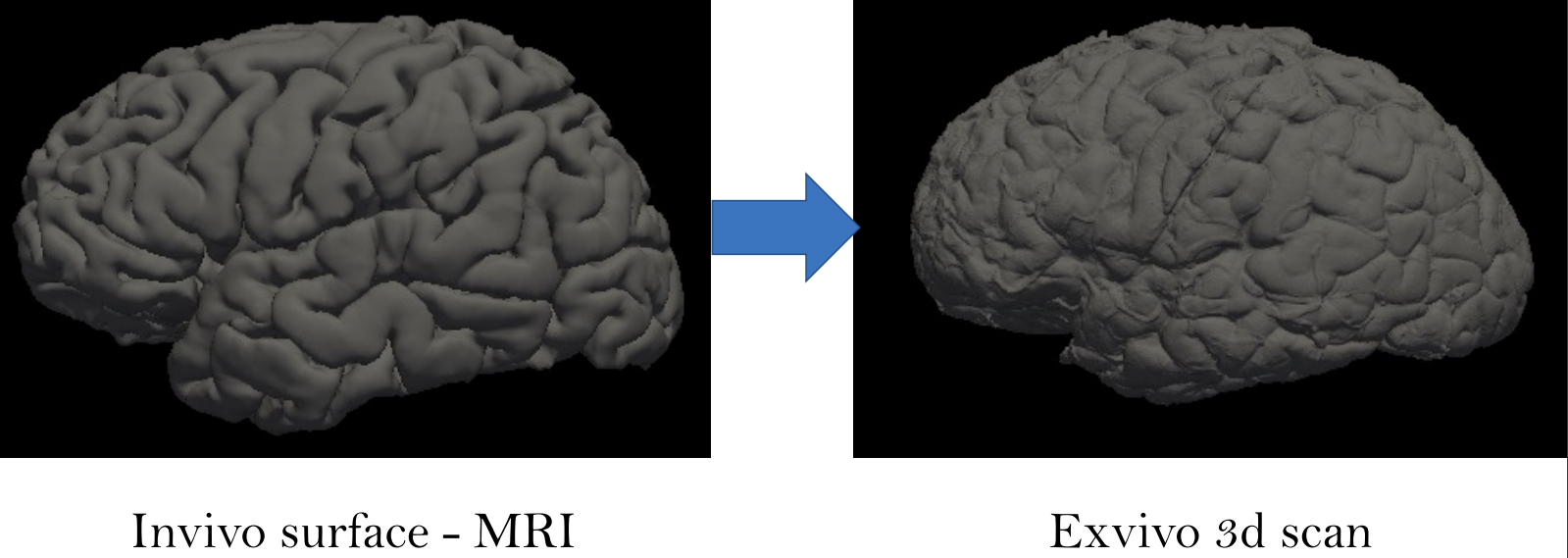
Ex-vivo surface mesh reconstruction from in-vivo FreeSurfer meshes is a process used to construct 3D models of neurological structures. This entails translating in-vivo MRI FreeSurfer meshes into higher-quality ex-vivo meshes. To accomplish this, the brain is first removed from the skull and placed in a solution to prevent deformation. A high-resolution MRI scanner produces a detailed 3D model of the brain’s surface. The in-vivo FreeSurfer mesh and the ex-vivo model are integrated for analysis and visualization, making this process beneficial for exploring brain structures, thereby helping scientists learn how it functions.
Figure 1 Converting in-vivo surface to exvivo 3d scan
2. Approach
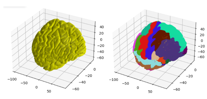
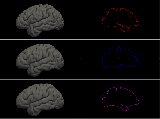
This project aims to construct anatomically accurate ex-vivo surface models of the brain from in-vivo FreeSurfer meshes. The source code for our project can be found in this GitHub repo. A software tool called FreeSurfer can be used to produce cortical surface representations from structural MRI data. However, because of distortion and shrinking, these meshes do not adequately depict the exact shape of the brain once it is removed from the skull. As a result, we propose a method for producing more realistic ex-vivo meshes for anatomical investigations and comparisons. For this task, we used five in-vivo meshes which were provided along with their annotations. Figure 2 shows a sample in-vivo mesh and its annotation.
Figure 2 Sample in-vivo mesh and its annotation
We attempted to solve this using two different spaces:
Volumetric space
Surface space
2.1. Volumetric Space
Our volumetric method consists of the following steps:
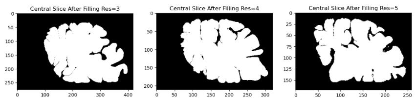
First, we fill in the high-resolution mesh into a 3D volume. This process ensures that the fine details of the cortical surface, such as gyri and sulci, are preserved while avoiding holes or gaps in the mesh. We performed the filling operation at three different resolutions which are 3,4 and 5 using FreeSurfer’s “mris_fill” command.
Figure 3 Central slice for different resolutions after filling
The deep sulci of the brain are then closed. Sulci are the grooves or fissures in the brain that separate the gyri or ridges. These sulci can sometimes be overly deep or too wide, affecting the quality of brain imaging or analysis. This step is necessary because in-vivo meshes often include open sulci which are not visible in the ex-vivo condition due to tissue collapse and folding. By closing the sulci, we can obtain a smoother and more compact mesh that resembles the ex-vivo brain surface.
Figure 4 Central slice for different resolutions after closing
Morphological operations are methods that change the shape or structure of a shape depending on a preset kernel or structuring element. There are a number of morphological operations, but we will concentrate on three here: dilation, fill and erode. Dilation extends an object’s borders by adding pixels to its edges. Fill adds pixels to the interior of an object to fill in any holes or gaps. Erode reduces the size of an object’s bounds by eliminating pixels from its edges. We can apply morphological operations to smooth out the brain surface and close the gaps to remedy this problem.
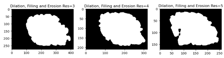
We used the following operations in a specified order to close the deep sulci of the brain: dilation, fill and erode. We first dilate the brain image to make the sulci smaller and less deep. The remaining spaces in the sulci are then filled to make them disappear. Finally, the brain image is eroded to recover its original size and shape. As a result, the brain surface is smoother and more uniform, with no deep sulci.
Figure 5 Central slice for different resolutions after dilation, filling, and erosion
The extraction of iso-surfaces from the three-dimensional volumetric data is accomplished using the well-known algorithm Marching Cubes, which results in a more uniform and accurate representation of the brain surface. This process transforms the three-dimensional volume into a surface mesh that can be visualized and examined.
Then we used the Gaussian smoothing algorithm in order to smooth the output of the marching cubes algorithm. In order to smooth an image, a Gaussian function is applied to each pixel using a Gaussian blur filter. Often employed in statistics, the normal distribution is mathematically described by a function called a Gaussian function. A Gaussian function in one dimension has the following form:
Figure 4 shows the visualization results of the reconstruction results before and after the application of Gaussian smoothing.
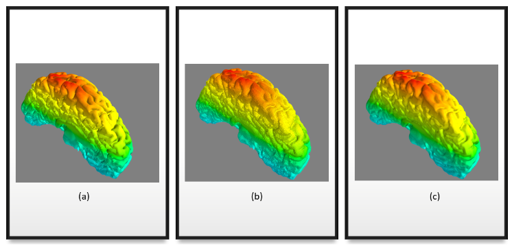
Figure 7 (a) original mesh, (b) reconstructed mesh using marching cubes without smoothing, (c) reconstructed mesh after smoothing.
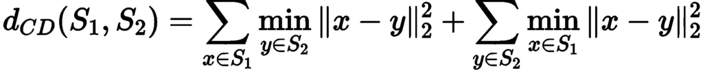
Finally, we used the density-aware chamfer distance to assess the quality of the reconstructed mesh. For comparing point sets, two popular metrics known as Chamfer Distance (CD) and Earth Mover’s Distance (EMD) are commonly used. While EMD focuses on global distribution and disregards fine-grained structures, CD does not take into account local density variations, potentially disregarding the underlying similarity between point sets with various density and structure features. We define the chamfer distance between two pointsets using the formula below:
From the reconstruction results, we can visually see that when the resolution increases the result is not so great. After performing the morphological operations we can see that the results for resolution of 5 still have some holes and the sulci is still deep. While for the lowest resolution of 3, we can see that the reconstruction is closer to ex-vivo than in-vivo. In order to validate our assumptions from the visualization, we computed the chamfer distance between the original mesh and the reconstructed mesh after the morphological operations are performed. The results after the calculation are summarized in Table 1.
Resolutions
N=10
N=100
N=1000
N=10000
3
4.15
7.62
76.26
274.73
4
5.66
10.09
42.92
182.66
5
4.53
8.60
33.19
168.83
Table 1 Chamfer distance for different resolutions
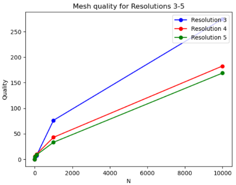
After getting the point clouds from both meshes, we only considered a subset of the vertices to compute the distance since considering the entire point cloud is computationally intensive and very slow. We took the number of vertices to be powers of 10. Then the point clouds were rescaled and normalized to be in the same space. From the results, we can conclude that the higher resolution has the lowest distance, while the lowest resolution has the highest distance. This is true from our observation that the highest resolution should be closer to the original mesh while the lowest resolution is further from it since it’s getting similar to an ex-vivo mesh. Figure 8 shows a plot of the mesh quality for the different resolutions, where the number of vertices is given on the x-axis and the distance is given on the y-axis.
Figure 8 Mesh quality for different resolutions
2.2. Surface-based approach
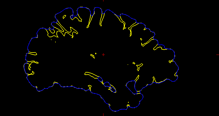
Sellán et al. demonstrate in “Opening and Closing Surfaces (2020)” that many regions don’t move when performing closing operations, and the output is curvature bound, as shown in Figure 9.
Figure 9 (yellow) Original outline, (blue) Closed outline
Therefore, Sellán et al. propose a bounded curvature-based flow for 3D surfaces that moves not curvature bound points in the normal direction by an amount proportional to their curvature.
As an alternative to the volumetric closing of the deep sulci of the brain, we applied the Sellán et al. method to close our surfaces. Figures 10 and 11 present the progressive closing of the mesh at each iteration until it converges.
Figure 10 Surface at each iteration of the closing flow
Figure 11 Outlining the difference at iterations 2, 4 and 6
2.3. Extracting External Surface
One other approach we tried to explore was focused on getting only the outer surface without all the grooves by post-processing the meshes reconstructed from the in-vivo reconstructed surface (Figure 12. a). So we followed the following steps:
Inflate the mesh by pushing each vertex in the direction of its normals. This results in the closing of all the grooves and only the external surface is directly visible. The inflated mesh is shown in Figure 12. b
Once we have this inflated surface, we need to retrieve only the externally visible surface. For this, we treat all the brain vertex as origins and shoot rays in the direction of vertex normals. The rays originating from vertices lying on the external surface do not hit any other surface, whereas the ones from the inside surface hit the external surface. Thus we can find and isolate the vertices lying on the surface. We reconstruct the surface using these extracted meshes using Poisson reconstruction. The reconstructed mesh is shown in Figure 12. c
Figure 12 Post-processing the meshes reconstructed from the in-vivo reconstructed surface
3. Future work
In this study, we presented a technique for reconstructing an ex-vivo mesh from an in-vivo mesh utilizing various methods. But there are still limitations and difficulties that we would like to address in our future studies. One of them is to mimic the effects of cuts and veins, which are common artifacts in histological images, on the surface of the brain. To achieve this, we intend to produce accurate displacement maps that can simulate the deformation of the brain surface as a result of these factors. Additionally, using displacement maps, we will investigate various techniques for producing random continuous curves on the 2D surface that can depict cuts and veins. Another challenge is to improve the robustness of our method to surface deformation caused by different slicing methods or imaging modalities. We also want to train deep learning networks such as GCN/DiffusionNet to segment different brain regions. We will investigate the use of chamfer distance as a loss function to measure the similarity between the predicted and ground truth segmentation masks, and to encourage smoothness and consistency of the segmentation results across different slices.
Fellows: Aditya Abhyankar, Munshi Sanowar Raihan, Shanthika Naik, Bereket Faltamo, Daniel Perazzo
Volunteer: Despoina Paschalidou
Mentor: Nicholas Sharp
I. Introduction
Triangular and tetrahedral meshes are central to geometry, we use them to represent shapes, and as bases to compute with. Many numerical algorithms only actually work well on meshes that have nicely-shaped triangles/tetrahedra, so we try very hard to generate meshes which simultaneously:
Represent the desired shape
Have nicely-shaped elements and
Perfectly interlock to cover the domain with no gaps or overlaps.
Yet, is point (3) really that important? What if instead we just sampled a soup of random nicely-shaped triangles, and didn’t worry about whether they fit together?
In this project we explore several strategies for generating such random meshes, and evaluate their effectiveness.
II. Algorithms
II.1. Triangle Sampling
Fig 1: The heat geodesic method fails if the triangles are isolated (left); but if the triangles share vertex entries, the heat method works even with gaps and intersections (right).
In random meshing, we are given the boundary of a shape (e.g. the polygon outline of a 2D figure) and the task is to generate random meshes to tessellate the interior. Here, we will focus mainly on the planar case, where we generate triangles with 2D vertex positions. We will test the generated meshes by running the Heat Method [2], a simulation-based algorithm for computing distance within a shape. The very first shape we tried to tessellate is a circular disk.
Since a circle is a convex shape, we can choose three random points inside the circle and any triangle is guaranteed to stay within the shape. But generating isolated triangles like these is not a good strategy, because downstream algorithms like the heat method rely on shared vertices to communicate across the mesh. Without shared vertices, it is equivalent to running the algorithm individually on a bunch of separate triangles one at a time.
Next strategy: At each vertex, consider generating n random triangles that are connected to other vertices within a certain radius. This ensures that the generated triangles share the same vertex entries. Even though these random triangles have many gaps and intersections, many algorithms are actually perfectly well-defined on such a mesh. To our surprise, the heat method was able to generate reasonable results even with these random soup of triangles (Fig 1).
II.2. Non-Convex Shapes
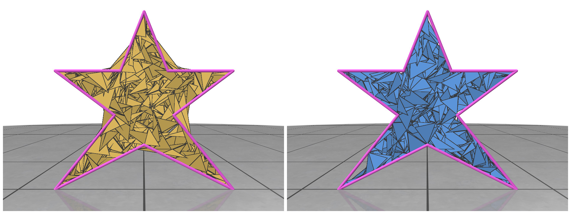
Fig 2: Random meshing of a non-convex star shape (left); mesh generated by rejection sampling of the triangles (right).
For non-convex shapes, if we try to connect any three points within the polygon, some of the triangles might fall outside of our 2D boundary. This is illustrated in Fig 2 (left). To circumvent this problem, we can do rejection sampling of the triangles. Every time we generate a new triangle, we need to test whether it is completely contained within the boundary of our polygon. If it’s not, we reject it from our face list and sample another one. After rejection, the random meshes seem to nicely follow the boundary. Rejection sampling makes our meshing algorithm a little slower, but it’s necessary to handle non-convex shapes.
II.3. Triangle Size
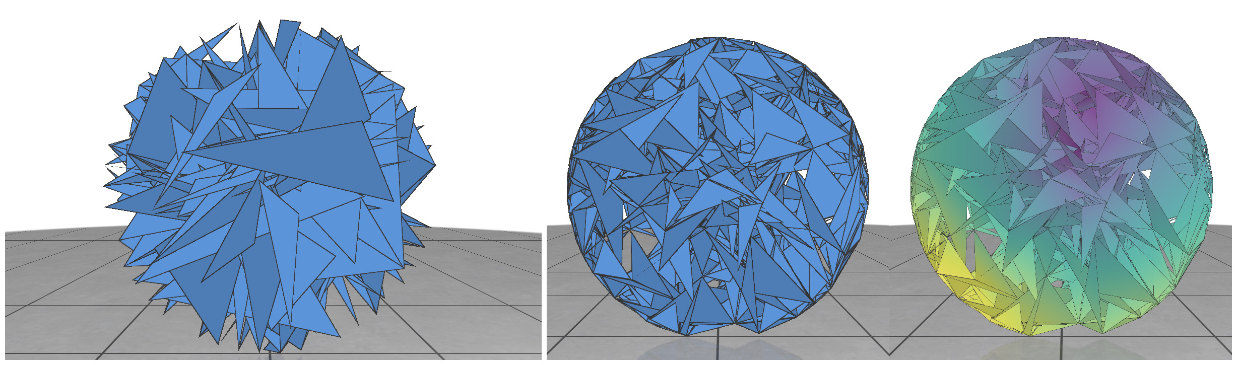
Fig 3: Random meshes with different triangle size (left) and the isolines of their geodesic distance from the source (right).
In random meshes, we find that the performance of the heat geodesic method is dependent on the size of the triangles. Since we are generating triangles by sampling points within a radius, we can make the triangles smaller or larger by controlling the radius of the circle. With decreasing triangle size, the distance computed by the heat method becomes more accurate. This is illustrated in Fig 3: as the triangles become smaller, the isolines look more precise. The number of triangles are kept fixed in all cases.
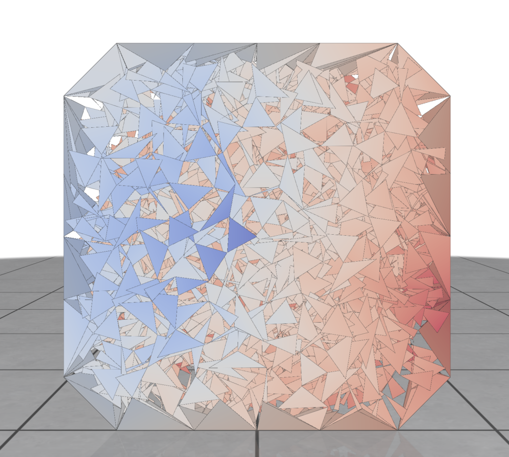
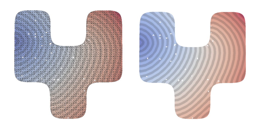
III. Visualizations and results
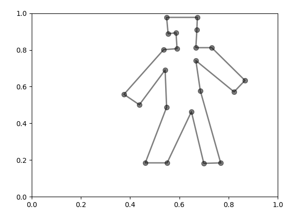
We created an interface to aid in the task of drawing different polygon shapes for visualization. As can be seen below, an example of a shape:
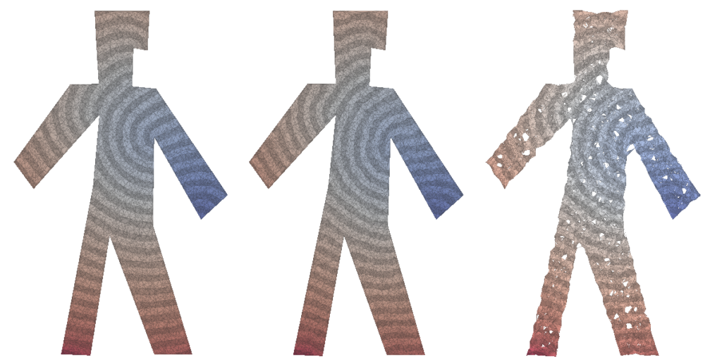
We can use one of our algorithms to plot various types of meshes with the distance function drawn by the heat equation. We put the visualization of these meshes bellow, where the leftmost is the mesh using Delaunay triangulation, the rightmost using random triangles and the center being using Delaunay triangulation but using the faces from the Delaunay triangulation for a better visualization.
In this case, with 5000 points sampled randomly, we have an error of 0.0002 compared with the values for the distance function compared with using the heat method.
IV. An Attempt at Random Walk Meshing
Another interesting meshing idea is spawning a single vertex somewhere in the interior of the shape, and then iteratively “growing” the mesh from there in the style of a random walk. At each iteration, every leaf vertex randomly spawns two more child vertices on the circumference of a circle surrounding it, which are used to form a new face. If any such spawning circle intersects with the boundary of the shape, we simply use the two vertices of the closest boundary edge instead to form the new face. We tried various types of random walk strategies, such as using correlated random walks with various correlation settings to mitigate clustering at the source vertex.
While this produced an interesting single component random mesh, the sparse connectivity made it a bad algorithm for the heat method, as triangle sequences that swiveled back around in the direction of the source vertex diffused heat backwards in that direction too.
This caused the distance computations to be inaccurate and rendered the other methods superior. We would like to explore this approach further though, as it might prove useful for other use-cases like physics simulations and area approximations. Random walks are very well studied in probability literature too, so deriving theoretical results for such algorithms seems like a very principled task.
V. Structure in Randomness
While sampling triangles within a radius gave a reasonable results upon calculating geodesic distance, we tried exploring ways to make it more structured. One such method we came with is grid sampling with triangulation within a neighborhood. The steps are as follows:
Uniformly sample points within a square grid enclosing the entire shape.
Eliminate points outside that fall out of the desired shape.
For each vertex within the shape, form a fan of triangles with its 1 ring neighborhood vertices.
These are the geodesic isolines on the triangular mesh obtained using the above method.
VI. Conclusion and Future Work
We present some examples of our random computation method working on 2D meshes for various different shapes. Aside from refining our algorithms and performing more experiments, one interesting avenue would be to perform experiments with tetrahedralization on 3D shapes. We have also done simple tests with current state-of-the-art tetrahedralization algorithms [3], the results are shown below. So, for future work, this would be a really interesting avenue. Another interesting avenue for theoretical work regarding random walk meshing would be computing how the density of triangles varies with iteration count and various degrees of correlation.
VII. References
[1] Shewchuk, Jonathan Richard. “Triangle: Engineering a 2D quality mesh generator and Delaunay triangulator.” Workshop on applied computational geometry. Berlin, Heidelberg: Springer Berlin Heidelberg, 1996.
[2] Crane, Keenan, Clarisse Weischedel, and Max Wardetzky. “The heat method for distance computation.” Communications of the ACM 60.11 (2017): 90-99.
[3] Hu, Yixin, et al. “Tetrahedral meshing in the wild.” ACM Trans. Graph. 37.4 (2018): 60-1.
[4] Hu, Yixin, et al. “Fast tetrahedral meshing in the wild.” ACM Transactions on Graphics (TOG) 39.4 (2020): 117-1.
Students: Tewodros (Teddy) Tassew, Anthony Ramos, Ricardo Gloria, Badea Tayea
TAs: Heng Zhao, Roger Fu
Mentors: Yingying Wu, Etienne Vouga
Introduction
Shape analysis has been an important topic in the field of geometry processing, with diverse interdisciplinary applications. In 2005, Reuter, et al., proposed spectral methods for the shape characterization of 3D and 2D geometrical objects. The paper demonstrates that the Laplacian operator spectrum is able to capture the geometrical features of surfaces and solids. Besides, in 2006, Reuter, et al., proposed an efficient numerical method to extract what they called the “Shape DNA” of surfaces through eigenvalues, which can also capture other geometric invariants. Later, it was demonstrated that eigenvalues can also encode global properties like topological features of the objects. As a result of the encoding power of eigenvalues, spectral methods have been applied successfully to several fields in geometry processing such as remeshing, parametrization and shape recognition.
In this project, we present a discrete surface characterization method based on the extraction of the top smallest k eigenvalues of the Laplace-Beltrami operator. The project consists of three main parts: data preparation, geometric feature extraction, and shape classification. For the data preparation, we cleaned and remeshed well-known 3D shape model datasets; in particular, we processed meshes from ModelNet10, ModelNet40, and Thingi10k. The extraction of geometric features is based on the “Shape DNA” concept for triangular meshes which was introduced by Reuter, et al. To achieve this, we computed the Laplace-Beltrami operator for triangular meshes using the robust-laplacian Python library.
Finally, for the classification task, we implemented some machine learning algorithms to classify the smallest k eigenvalues. We first experimented with simple machine learning algorithms like Naive Bayes, KNN, Random Forest, Decision Trees, Gradient Boosting, and more from the sklearn library. Then we experimented with the sequential model Bidirectional LSTM using the Pytorch library to try and improve the results. Each part required different skills and techniques, some of which we learned from scratch and some of which we improved throughout the two previous weeks. We worked on the project for two weeks and received preliminary results. The GitHub repo for this project can be found in this GitHub repo.
Data preparation
The datasets used for the shape classification are:
1. ModelNet10: The ModelNet10 dataset, a subset of the larger ModelNet40 dataset, contains 4,899 shapes from 10 categories. It is pre-aligned and normalized to fit in a unit cube, with 3,991 shapes used for training and 908 shapes for testing.
2. ModelNet40: This widely used shape classification dataset includes 12,311 shapes from 40 categories, which are pre-aligned and normalized. It has a standard split of 9,843 shapes for training and 2,468 for testing, making it a widely used benchmark.
3. Thingi10k: Thingi10k is a large-scale dataset of 10,000 models from thingiverse.com, showcasing the variety, complexity, and quality of real-world models. It contains 72 categories that capture the variety and quality of 3D printing models.
For this project, we decided to use a subset of the ModelNet10 dataset to perform some preprocessing steps on the meshes and apply a surface classification algorithm due to the number of classes it has for analysis. Meanwhile, the ModelNet10 dataset is unbalanced, so we selected 50 shapes for training and 25 for testing per class.
Moreover, ModelNet datasets do not fully represent the surface representations of objects; self-intersections and internal structures are present, which could affect the feature extraction and further classification. Therefore, for future studies, a more careful treatment of mesh preprocessing is of primary importance.
Preprocessing Pipeline
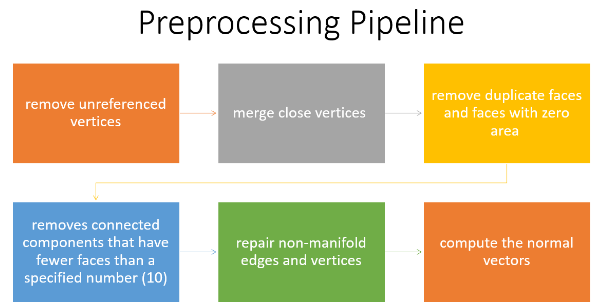
After the dataset preparation, the preprocessing pipeline consists of some steps to clean up the meshes. These steps are essential to ensure the quality and consistency of the input data, and to avoid errors or artifacts. We used the PyMeshLab library, which is a Python interface to MeshLab, for mesh processing. The pipeline consists of the following steps:
1.Remove unreferenced vertices: This method gets rid of any vertices that don’t belong to a face.
2. Merge nearby vertices: This function combines vertices that are placed within a certain range (i.e., ε = 0.001).
3.Remove duplicate faces and faces with zero areas: It eliminates faces with the same features or no area.
4. Removes connected components that have fewer faces than a specified number (i.e. 10): The effectiveness and accuracy of the model can be enhanced by removing isolated mesh regions that are too small to be useful.
5.Repair non-manifold edges and vertices: It corrects edges and vertices that are shared by more than two faces, which is a violation of the manifold property. The mesh representation can become problematic with non-manifold geometry.
6.Compute the normal vectors: The orientation of the adjacent faces is used to calculate the normal vectors for each mesh vertex.
These steps allow us to obtain clean and consistent meshes that are ready for the remeshing process.
Figure 1 Preprocessing Pipeline
Adaptive Isotropic Remeshing
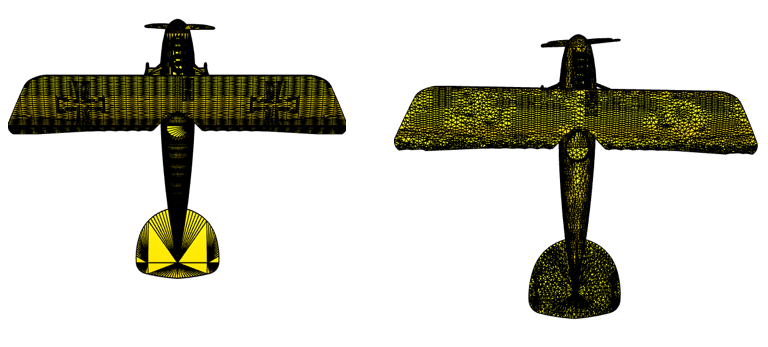
The quality of the meshes is one of the key problems with the collected 3D models. When discussing triangle quality, it’s important to note that narrow triangles might result in numerical inaccuracies when the Laplace-Beltrami operator is being computed. In that regard, we remeshed each model utilizing adaptive isotropic remeshing implemented in PyMeshLab. Triangles with a favorable aspect ratio can be created using the procedure known as isotropic remeshing. In order to create a smooth mesh with the specified edge length, the technique iteratively carries out simple operations like edge splits, edge collapses, and edge flips.
Adaptive isotropic remeshing transforms a given mesh into one with non-uniform edge lengths and angles, maintaining the original mesh’s curvature sensitivity. It computes the maximum curvature for the reference mesh, determines the desired edge length, and adjusts split and collapse criteria accordingly. This technique also preserves geometric details and reduces the number of obtuse triangles in the output mesh.
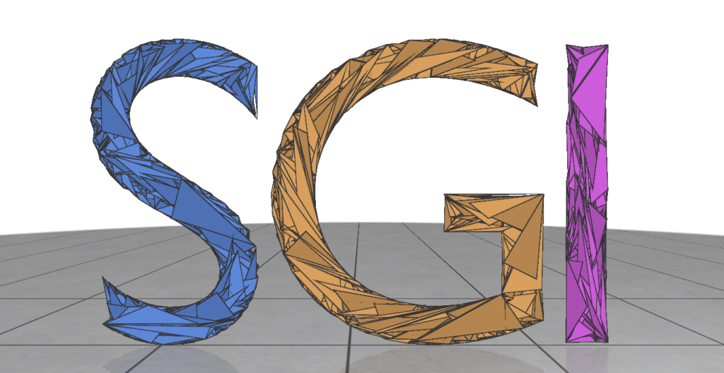
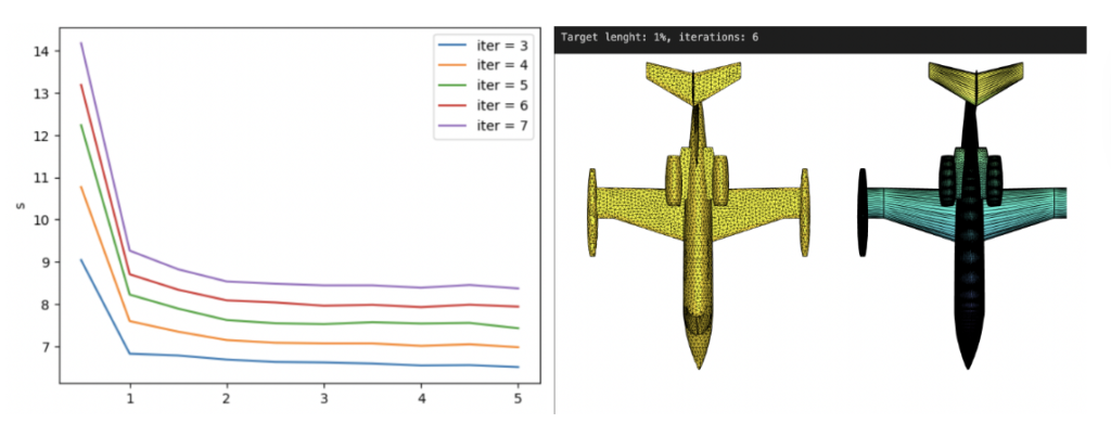
We applied the PyMeshLab function ms.meshing_isotropic_explicit_remeshing() to remesh the ModelNet10 dataset for this project. We experimented with different parameters of the isotropic remeshing algorithm from PyMeshLab to optimize the performance. The optimal parameters for time, type of remesh, and triangle quality were iterations=6, adaptive=True, and targetlen=pymeshlab.Percentage(1) respectively. The adaptive=True parameter enabled us to switch from uniform to adaptive isotropic remeshing. Figure 3 illustrates the output of applying adaptive remeshing to the airplane_0045.off mesh from the ModelNet40 training set. We also tried the pygalmesh.remesh_surface() function, but it was very slow and produced unsatisfactory results.
Figure 3 Plot for time vs target length (left) and the yellow airplane is the re-meshing result for parameter values of Iterations = 6 and targetlen = 1% while the blue airplane is the original mesh (right).
The Laplace-Beltrami Spectrum Operator
In this section, we introduce some of the basic theoretical foundations used for our characterization. Specifically, we define the Laplacian-Beltrami operator along with some of its key properties, explain the significance of the operator and its eigenvalues, and display how it has been implemented in our project.
Definition and Properties of the Laplace-Beltrami Operator
The Laplacian-Beltrami operator, often denoted as Δ, is a differential operator which acts on smooth functions on a Riemannian manifold (which, in our case, is the 3D surface of a targeted shape). The Laplacian-Beltrami operator is an extension of the Laplacian operator in Euclidean space, adjusted for curved surfaces on the manifold. Mathematically, the Laplacian-Beltrami operator acting on a function on a manifold is defined using the following formula:
where ∂idenotes the i-th partial derivative, g is the determinant of the metric tensor gij of the manifold and gijis the inverse of the metric tensor.
The Laplacian-Beltrami operator serves as a measure of how the value of f at a point deviates from its average value within infinitesimally small neighborhoods around that point. Therefore, the operator can be adopted to describe the local geometry of the targeted surface.
The Eigenvalue Problem and Its Significance
Laplacian-Beltrami operator is a second-order function applied to a surface, which could be represented as a matrix whose eigenvalues/eigenvectors provide information about the geometry and topology of a surface.
The significance of the eigenvalue problem as a result of applying the Laplace-Beltrami Operator includes:
Functional Representation. The eigenfunctions corresponding to a particular geometric surface form an orthonormal basis of all functions on the surface, providing an efficient way to represent any function on the surface.
Surface Characterization. A representative feature vector containing the eigenvalues creates a “Shape-DNA” of the surface, which captures the most significant variations in the geometry of the surface.
Dimensionality Reduction. Using eigenvalues can effectively reduce the dimensionality of the data used, aiding in more efficient processing and analysis.
Feature Discrimination. The geometric variations and differences between surfaces can be identified using eigenvalues. If two surfaces have different eigenvalues, they are likely to have different geometric properties. Surface eigenvalue analysis can be used to identify features that are unique to each surface. This can be beneficial in computer graphics and computer vision applications where it is necessary to distinguish between different surfaces.
Discrete Representation of Laplacian-Beltrami Operator
In the discrete setting, the Laplacian-Beltrami operator is defined on the given meshes. The Discrete Laplacian-Beltrami operator L can be defined and computed using different approaches. An often-used representation is using the cotangent matrix defined as follows:
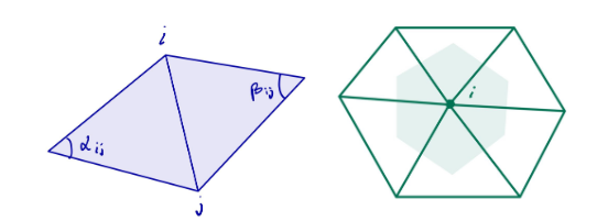
Then L = M-1C where M is the diagonal mass matrix whose i-th entry is the shaded area as shown in Figure 4 for each vertex i. The Laplacian matrix is a symmetric positive-semidefinite matrix. Usually, L is sparse and stored as a sparse matrix in order not to waste memory.
Figure 4 (Left) Definition of edge i-j and angles for a triangle mesh. (Right) Representation of Voronoi area for vertex vi.
A Voronoi diagram is a mathematical method for dividing a plane into areas near a collection of objects, each with its own Voronoi cell. It contains all of the points that are closer to it than any other object. Since its origin, engineers have utilized the Delaunay triangulation to maximize the minimum angle among possible triangulations of a fixed set of points. In a Voronoi diagram, this triangulation corresponds to the nerve cells.
Experimental Results
In our experiments, we rescaled the vertices before computing the cotangent Laplacian. Rescaling mesh vertices changes the size of an object without changing its geometry. This Python function rescales a 3D point cloud by translating it to fit within a unit cube centered at the origin. It then scales the point cloud to have a maximum norm of 1, ensuring its center is at the origin. The function then finds the maximum and minimum values of each dimension in the input point cloud, computes the size of the point cloud in each dimension, and computes a scaling factor for each dimension. The input point cloud is translated to the center at the origin and scaled by the maximum of these factors, resulting in a point cloud with a maximum norm of 1.
Throughout this project, we used the robust-laplacian Python package to compute the Laplacian-Beltrami operator. This library deals with point clouds instead of triangle meshes. Moreover, the package can handle non-manifold triangle meshes by implementing the algorithm described in A Laplacian for Nonmanifold Triangle Meshes by Nicholas Sharp and Keenan Crane.
For the computation of the eigenvalues, we used the SciPy Python library. Let’s recall the eigenvalue problem Lv = λv, where λ is a scalar, and v is a vector. For a linear operator L, we called λ eigenvalue and v eigenvector respectively. In our project, the smallest keigenvalues and eigenfunctions corresponding to 3D surfaces formed feature vectors for each shape, which were then used as input of machine learning algorithms for tasks such as shape classification.
Surface Classification
The goal of this project was to apply spectral methods to surface classification using two distinct datasets: a synthetic one and ModelNet10. We used the Trimesh library to create some basic shapes for our synthetic dataset and performed remeshing on each shape. This was a useful step to verify our approach before working with more complicated data. The synthetic data had 6 classes with 50 instances each. The shapes were Annulus, Box, Capsule, Cone, Cylinder, and Sphere. We computed the first 30 eigenvalues on 50 instances of each class, following the same procedure as the ModelNet dataset so that we could compare the results of both datasets. We split the data into 225 training samples and 75 testing samples.
For the ModelNet10 dataset, we selected 50 meshes for the training set and 25 meshes for the testing set per class. In total, we took 500 meshes for the training set and 250 meshes for the testing set. After experimenting with different machine learning algorithms, the validation results for both datasets are summarized below in Table 1. The metric used for the evaluation procedure is accuracy.
Models
Accuracy for Synthetic Dataset
Accuracy for ModelNet 10
KNN
0.49
0.31
Random forest
0.69
0.33
Linear SVM
0.36
0.11
RBF SVM
0.60
0.10
Gaussian Process
0.59
0.19
Decision Tree
0.56
0.32
Neural Net
0.68
0.10
AdaBoost
0.43
0.21
Naive Bayes
0.23
0.19
QDA
0.72
0.21
Gradient Boosting
0.71
0.31
Table 1 Accuracy for synthetic and ModelNet10 datasets using different machine learning algorithms.
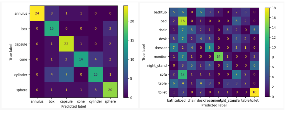
From Table 1 we can observe that the decision tree, random forest, and gradient boosting algorithms performed well on both datasets. These algorithms are suitable for datasets that have graphical features. We used the first 30 eigenvalues on 50 samples of each class for both the ModelNet and synthetic datasets, ensuring a fair comparison between the two datasets. Figure 5 shows the classification accuracy for each class using the confusion matrix.
Figure 5 Confusion matrix using Random Forest on the synthetic dataset (left) and ModelNet10 dataset (right).
We conducted two additional experiments using deep neural networks implemented in Pytorch, besides the machine learning methods we discussed before. The first experiment involved a simple MLP model consisting of 5 fully connected layers, each with the Batch Norm and ReLU activation functions. The model achieved an accuracy of 57% on the synthetic dataset and 15% on the ModelNet10 dataset for the testing set. The second experiment used a sequential model called Bidirectional LSTM with two layers. The model achieved an accuracy of 34% for the synthetic dataset and 33% for the ModelNet10 dataset based on the testing set. These are reasonable results since the ModelNet dataset contains noise, artifacts, and flaws, potentially affecting model accuracy and robustness. Examples include holes, missing components, uneven surfaces, and most importantly, the interior structures. All of these issues could potentially impact the overall performance of the models, especially for our classification purposes. We present the results in Table 2. The results indicate that the MLP model performed well on the synthetic dataset while the Bi-LSTM model performed better on the ModelNet10 dataset.
Models
Accuracy for Synthetic Dataset
Accuracy for ModelNet 10
MLP
0.57
0.15
Bi-LSTM
0.34
0.33
Table 2 Accuracy for synthetic and ModelNet10 datasets using deep learning algorithms.
Future works
We faced some challenges with the ModelNet10 dataset. The dataset had several flaws that resulted in lower accuracy when compared to the synthetic dataset. Firstly, we noticed some meshes with disconnected components, which caused issues with the computation of eigenvalues, since we would get one zero eigenvalue for each disconnected component, lowering the quality of the features computed for our meshes. Secondly, these meshes had internal structures, i.e., vertices inside the surface, which also affected the surface recognition power of the computed eigenvalues, as well as other problems related to self-intersections and non-manifold edges.
The distribution of eigenvalues in a connected manifold is affected by scaling. The first-keigenvalues are related to the direction encapsulating the majority of the manifold’s variation. Scaling by α results in a more consistent shape with less variation along the first-k directions. On the other hand, scaling by 1/α causes the first-k eigenvalues to grow by α2, occupying a higher fraction of the overall sum of eigenvalues. This implies a more varied shape with more variance along the first-k directions.
To address the internal structures problem, we experimented with several state-of-the-art surface reconstruction algorithms for extracting the exterior shape and removing internal structures using the Ball Pivoting, Poisson Distribution methods from the Python PyMeshLab library, and Alpha Shapes. One of the limitations of ball pivoting is that the quality and completeness of the output mesh depend on the choice of the ball radius. The algorithm may miss some parts of the surface or create holes if the radius is too small. Conversely, if the radius is too large, the method could generate unwanted triangles or smooth sharp edges. Ball pivoting also struggles with noise or outliers and can result in self-intersections or non-manifold meshes.
By using only vertices to reconstruct the surface, we significantly reduced the computational time but the drawback was that the extracted surface was not stable enough to recover the entire surface. It also failed to remove the internal structures completely. In future work, we intend to address this issue and create an effective algorithm that can extract the surface from this “noisy” data. For this issue, implicit surface approaches show great promise.
References
Reuter, M., Wolter, F.-E., & Niklas Peinecke. (2005). Laplace-spectra as fingerprints for shape matching. Solid and Physical Modeling. https://doi.org/10.1145/1060244.1060256
Reuter, M., Wolter, F.-E., & Niklas Peinecke. (2006). Laplace–Beltrami spectra as “Shape-DNA” of surfaces and solids. Computer Aided Design, 38(4), 342–366. https://doi.org/10.1016/j.cad.2005.10.011
Reuter, M., Wolter, F.-E., Shenton, M. E., & Niethammer, M. (2009). Laplace–Beltrami eigenvalues and topological features of eigenfunctions for statistical shape analysis. 41(10), 739–755. https://doi.org/10.1016/j.cad.2009.02.007
Nealen, A., Igarashi, T., Sorkine, O., & Alexa, M. (2006). Laplacian mesh optimization. Conference on Computer Graphics and Interactive Techniques in Australasia and Southeast Asia. https://doi.org/10.1145/1174429.1174494
By SGI Fellows: Anna Cole, Francisco Unai Caja López, Matheus da Silva Araujo, Hossam Mohamed Saeed
I. Introduction
In this project, mentored by Professor Paul Kry, we are exploring properties and applications of multiresolution surface representations: surface meshes with different complexities and details that represent the same underlying surface.
Frequently, the digital representation of intricate and detailed surfaces requires huge triangle meshes. For instance, the digital scan of Michelangelo’s statue of David [9] contains over 1 billion polygon faces and requires 32 GB of memory. The high level of complexity makes it costly to store and render the surface. Furthermore, applying standard geometry processing algorithms on such complex meshes requires huge computational resources. An alternative consists in representing the underlying surface using hierarchy of meshes, also known as multiresolution representations [2]. Each successive level of the hierarchy uses a mesh with lower geometric complexity while representing the same smooth surface. A hierarchy of meshes allows to represent surfaces at different resolutions, which is critical to handle complex geometric models. This form of representation provides efficiency and scalability for rendering and processing of complex surfaces, because the level of detail of the surface can be adjusted based on the hardware available. Figure 1 shows one example of a hierarchy of meshes. In this project we explore the construction of hierarchical representations of surface meshes combined with correspondences between different levels of the hierarchy.
Figure 1: a hierarchy of meshes built using mesh simplification.
One critical point of this construction is a mapping between meshes at different levels. Liu et al. 2020 [7] proposes a bijective map, named successive self-parameterization, that allows to correspond coarse and fine meshes on the multiresolution hierarchy. To build this mapping, successive self-parameterization requires a (i) mesh simplification algorithm to build the hierarchy of meshes and (ii) a conformal parameterization to map meshes on successive refinement levels to a common space. Our goal for this project is to investigate different applications of this mapping. In the next sections, we detail the algorithms to construct the hierarchy and the successive self-parameterization.
II. Mesh simplification
II.1. Mesh simplification using quadric error
The mesh simplification algorithm studied was introduced in Garland and Heckbert 1997 [6] and is quite straightforward: it consists in collapsing various edges of the mesh sequentially. Specifically, in each iteration, two neighboring vertices \(v_i\) and \(v_j\) will be chosen and replaced by a single vertex \(\overline{v}\). The new vertex \(\overline{v}\) will inherit all neighbors of \(v_i\) and \(v_j\). In Animation 1 it is possible to see the possible result of two edge collapses in a triangle mesh.
Animation 1: consecutive edge collapses in a triangle mesh.
Suppose we have decided to collapse edge \((v_i,v_j)\). Then, \(\overline{v}\) is found as the solution of a minimization problem. For each vertex \(v_i\) we define a matrix \(Q_i\) so that \(v^TQ_iv\), with \(v=[v_x, v_y, v_z, 1]\), gives a measure of how far \(v\) is from \(v_i\). We choose \(\overline{v}\) minimizing \(v^T(Q_i+Q_j)v\). As for the choice of the \(Q\) matrices, we consider:
To each vertex \(v_i\) we associate the set of planes corresponding to faces that contain \(v_i\) and denote it \(\mathcal{P}(v_i)\).
For each face of the mesh we consider \(p=[a,b,c,d]^T\) such that \(v^Tp=0\) is the equation of the plane and \(a^2+b^2+c^2=1\). This allows us to compute the distance from a point \(v=[v_x,v_y,v_z,1]\) to the plane as \(\vert v^Tp \vert\).
Then, the sum of the squared distances from \(v\) to each plane in \(\mathcal{P}(v_i)\) would be
Finally, we decide which edge to collapse by choosing \((v_i,v_j)\) minimizing the error \(\overline{v}^T(Q_i+Q_j)\overline{v}\). For the following iterations, \(\overline{v}\) is assigned the matrix \(Q_i+Q_j\). Animations 2 and 3 illustrates the process of mesh simplification using quadric error.
Animation 2: mesh simplification of Spot.
Animation 3: mesh simplification of Fennec Fox.
The algorithm can also run on meshes with boundaries. In Animation 4 we chose not to collapse boundary edges, which allows the boundaries to be preserved.
Animation 4: simplification of a mesh with boundaries. In this case, the boundary of the mesh is preserved.
II.2. Manifoldness and edge collapse validation
There are a variety of issues that can occur if we collapse each edge only based on the error quadrics \(Q_i+Q_j\). This is because the error quadric is only concerned with the geometry of the meshes but not the topology. So we needed to implement some connectivity checks to make sure the edge collapse wouldn’t result in a non-manifold case or change the topology of the mesh.
This can be visualized in Animation 5, where collapsing an interior edge consisting of two boundary vertices can create a non-manifold edge (or vertex). Another problematic case is collapsing an edge with its two vertices sharing more than two neighboring vertices, which would break manifoldness. We followed the criteria described in Liu et al. 2020 [7] and Hoppe el al. 1993 [5] to guarantee an manifold input mesh stays manifold after each collapse. Also, we added the condition where we compute the Euler characteristic \(\chi(M)\) before and after the collapse and if there is a change, we revert back and choose a different edge. In case all remaining edges are not valid for the collapse operation, we simply stop the collapsing process and move on to the next step.
Animation 5: examples of valid edge collapses (left and center figures, in blue) and an example of an edge collapse that generates non-manifold elements (right figure, in orange).
III. Mesh parameterization
Mesh parameterization deals with the problem of mapping a surface to the plane. In our case, the surface is represented by a triangle mesh. This means that for every vertex of the triangle mesh we find corresponding coordinates on the 2D plane. More precisely, given a triangle mesh \(\mathcal{M}\), with a set of vertices \(\mathcal{V}\) and a set of triangles \(\mathcal{T}\), the mesh parameterization problem is concerned with finding a map \(f: \mathcal{V} \rightarrow \Omega \subset \mathbb{R}^{2}\). The effect of this mapping can be seen in Animation 6, where one 3D mesh is flattened to the 2D plane.
Animation 6: a triangle mesh embedded in \(\mathbb{R}^{3}\) is flattened to the 2D plane using a mesh parameterization algorithm.
This mapping enables all sorts of interesting applications. The most famous one is texture mapping: how to specify texture coordinates for each vertex of a triangle mesh such that you can map a region of an image to the mesh? Other applications include conversion of triangle meshes into parametric surfaces [11] e.g., T-Splines or NURBS and computational fabrication [12]. In this section we won’t give all the details about this field, but rather will focus on the aspects relevant to build mappings between meshes of different refinement levels on the hierarchical surface representation. We refer the interested reader to Hormann et al. 2007 [10] for an extensive treatment.
There are many different possibilities to define the mapping from the surface to the plane. However, this mapping usually introduces undesirable distortions. Depending on the construction used, the map may preserve areas, but not angles or orientations; conversely, it may preserve angles but not areas and lengths. This can be seen in Figure 2, where we can visualize angles and area distortions in the parameterized mesh.
Figure 2 : given a triangle mesh (left), we can map it to the 2D plane (center and right). This mapping can introduce angle distortions (center) and area distortions (right).
To create maps between meshes of different levels, Liu et al. 2020 [7] uses conformal mappings, which are maps that preserve angles. Conformal mappings are efficient to compute and provide theoretical guarantees, making it a common choice for many geometry processing tasks.
A conformal map is characterized by the Cauchy-Riemann equations:
Conformal mappings also have a strong connection with complex analysis, which leads to an alternative but equivalent formulation of the problem.
For arbitrary triangle meshes it is impossible to find an exact conformal mapping; only developable meshes (i.e., meshes with zero Gaussian curvature at every point) can be conformally parameterized. In most cases, this restriction is too severe. To work around this, it is possible to build a conformal mapping satisfying the previous equations as close as possible. In other words, we can associate it with an energy function to find the mapping that better approximates a conformal mapping using a least squares formulation:
where \(S\) is the smooth surface represented by a triangle mesh \(\mathcal{M}\).
On a triangle mesh, the functions \(u(x, y), v(x,y)\) can be written with respect to the local orthonormal coordinate system of the triangle. Since the triangle mesh is a piecewise linear surface, the gradient of a function defined over the mesh is constant with respect to each triangle. This makes it possible to find the mapping that better approximates the Cauchy-Riemann equations for each triangle of the mesh. Hence, in this discrete setting, the previous equation can be rewritten as follows
where \(A_{t}\) denotes the area of each triangle with vertices represented by \((i, j, k)\). The solution of the discrete conformal energy described above are the coordinates \((u, v)\) in the 2D plane for each vertex of each triangle \(t\) in the set of triangles \(\mathcal{T}\) of the mesh \(\mathcal{M}\). More details can be found in Lévy et al. 2002 [4] and Desbrun et al. 2002 [13].
However, the trivial solution for this equation would be to set all coordinates \((u, v)\) to the same point and the energy would be minimized, which is not what we want. Therefore, to prevent this case, it is necessary to fix or pin two arbitrary vertices to arbitrary positions in the plane. This restriction generates a least squares problem with a unique solution. The choice of the vertices to be fixed is arbitrary but can have impact on the quality and numerical stability of the parameterization. For instance, there can be arbitrary area distortions depending on the vertices that are fixed. To prevent the problem of the trivial solution while preserving numerical stability, an alternative strategy is proposed by Mullen et al. 2008 [3] in which the system is reformulated to an equivalent eigendecomposition problem which avoid the need to pin any vertex.
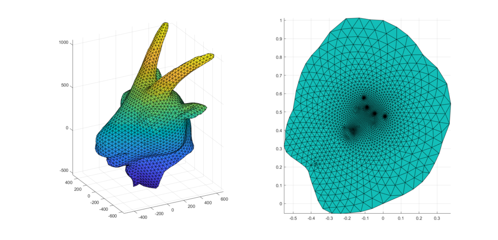
Figure 3 illustrates the least squares conformal mapping obtained for a triangle mesh with boundaries. Notice that the map obtained doesn’t necessarily preserve areas and lengths. Furthermore, as can be seen in the right plot of the figure, lots of details are grouped around tiny regions in the interior of the parameterized mesh.
Figure 3: a triangle mesh (left) and the resulting parameterized mesh in the plane (right).
This algorithm is a central piece to create a bijective map between meshes on different levels of the hierarchy.
IV. Successive self-parameterization
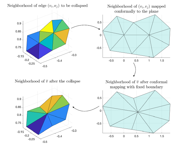
For each edge collapse, we use this procedure to create a bijective mapping between the original mesh, called \(\mathcal{M}^L\), and the mesh after an edge collapse, \(\mathcal{M}^{L-1}\). To construct a mapping from our coarsest mesh to finest mesh, we used spectral conformal parameterization as described in Mullen et al. 2008 [3] and build a successive mapping following the same procedure as Liu et al. 2020 [7]. As mentioned in the previous section, conformal mapping is a parameterization method that preserves angles. For a single edge collapse, \(\mathcal{M}^L\) and \(\mathcal{M}^{L-1}\) are the same except for the neighborhood of the collapsed edge. Therefore, if \((v_i,v_j)\) is the edge to be collapsed, we only need to build a mapping from the neighborhood of \((v_i,v_j)\) in \(\mathcal{M}^L\) to the neighborhood of \(\overline{v}\) in \(\mathcal{M}^{L-1}\). We do this in three steps:
We first map the neighborhood of \((v_i,v_j)\) to the plane via conformal mapping.
A key observation here is that the neighborhood of \(\overline{v}\in\mathcal{M}^{L-1}\) has the same boundary as the neighborhood of \((v_i,v_j)\) before the collapse. We then do a conformal mapping of the neighborhood of \(\overline{v}\in\mathcal{M}^{L-1}\) fixing the boundary so that the resulting 2D region is the same as before.
Now we map points between the 3D neighborhoods using the shared 2D domain.
This process is illustrated in Figure 4.
Figure 4: a triangle mesh before and after the collapse (left column) and their corresponding parameterizations (right column). By mapping the mesh before and after the collapse to the plane, it is possible to create a bijective mapping between the two meshes.
We repeat this process successively for a certain number of collapses to arrive at the desired, coarsest mesh. We refer to the combination of these methods as successive self-parameterization, as described in Liu et al. 2020 [7]. In the implementation of our algorithm, we ran into problems with overlapping faces and badly shaped, skinny triangles. We discuss the mitigation of these problems in the next section.
V. Testing And Improvements
In each part of the project, we always tried to test and potentially improve its results. These helped improve the final output as discussed in Section VI – Results.
V.1. Quality checks for avoiding skinny triangles
To help solve the problem of skinny triangles, we implemented a quality check on the triangles of our mesh post-collapse using the following formula:
Here \(A\) is the area of a triangle, \(l\) are the lengths of the triangle edges, and \(i,j,k\) represent the indices of the vertices on the triangle. Values of \(Q\) closer to 1 indicate a high quality triangle, while values nearing 0 indicate a degenerate, poor quality triangle. We implemented a test that undoes a collapse if any of the triangles generated have a low value of \(Q_{ijk}\). Figure 5 shows an image with faces of varying quality. Red indicates low quality while green indicates high quality.
Figure 5: visualization of the quality of each triangle in a triangle mesh. A red triangle represents bad quality while a green triangle represents good quality.
V.2. The Delaunay Condition and Edge flips for avoiding skinny triangles
After testing the pipeline on multiple meshes and with different parameters, we realized that there was one issue. While the up-sampled mesh had good geometric quality (due to successive self-parameterization), the triangle quality was not very good. This is because the edge collapses can generally produce some skinny triangles.
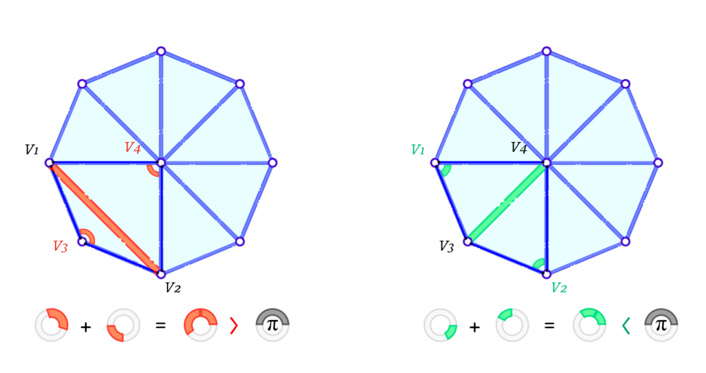
To solve this, we implemented a local edge flip after each edge collapse. In that case, we check for edges that don’t satisfy the Delaunay Condition. The Delaunay condition is a good way to improve the triangle angles by penalizing obtuse angles.
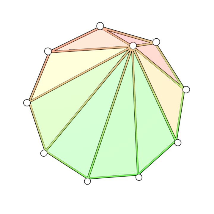
Figure 6: example of a mesh that does not satisfy the Delaunay condition (left) and of a mesh that does satisfy the Delaunay condition (right).
Figure 6 illustrates two cases where the left one violates the Delaunay condition while the one on the right satisfies it. Formally, for a given interior edge \(e_{1-2}\) connecting the vertices \(v_1\) and \(v_2\), and having \(v_3\) and \(v_4\) opposite to it on each of its 2 faces, it satisfies the condition if and only if the sum of the 2 opposite interior angles is less than or equal to \(\pi\). In other words:
As this makes it very unlikely to have obtuse angles, it eliminates some cases of skinny triangles. It is important to note that a skinny triangle can be produced even if all angles are acute, as one of them can be a very small angle. This is another case of skinny triangles but we have other checks mentioned before to help avoid such cases.
Figure 7: given an initial mesh (left), the edge collapse may generate skinny triangles (center). The edges of the triangles that violate the Delaunay condition are flipped (right).
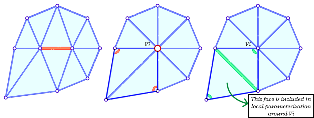
The edge flips are implemented right before the self-parameterization part. This is to improve triangle quality after each collapse. The candidate edges for a flip are only the ones that are connected to the vertex resulting from the collapse. We also need a copy of the face list before the flip to ensure the neighbourhood is consistent before and after the collapse when we go into the self-parameterization stage. Figure 7 shows an example of a consistent neighbourhood before the collapse, after the edge collapse and after the edge flip (in that order). We need to consider the face that is not any more a neighbor to the vertex to have a consistent mapping.
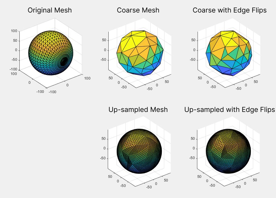
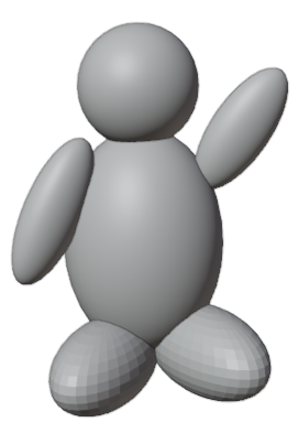
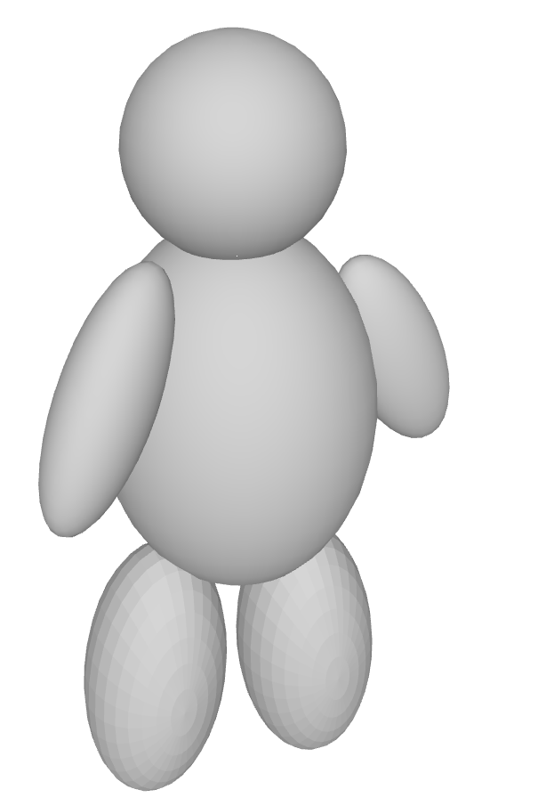
The addition of edge flips improved the triangle quality of the final mesh (after re-sampling for remeshing). Figure 8 shows an example of this on a UV sphere. A quantitative analysis of the improvement is also discussed in the Results section.
Figure 8: visual comparison between the results of mesh simplification without edge flip (center column) and with edge flip (right column).
V.3. Preventing UV faces overlaps
According to Liu et al. 2020 [7], even with consistently oriented faces in the Euclidean and parameterized spaces, it is still possible that two faces overlap each other in the parameterized space. To prevent this artifact, the authors propose to check, in the UV domain, if an interior vertex of the edge to be collapsed has a total angle over \(2 \pi\). If this condition is satisfied, then the edge should not collapse. However, it may also be the case that the condition is satisfied after the collapse. In this case, this edge collapse must be undone and a different edge must be collapsed.
VI. Results
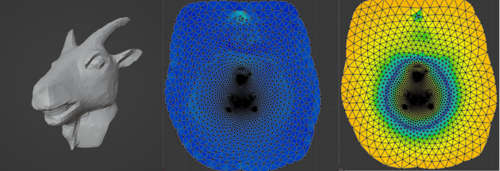
During this project we designed a procedure which can simplify any mesh via edge collapses as we have seen in all the animations. Figure 9 shows how well the coarse mesh approximates the original.
Figure 9: mean square distance between the original mesh and successive meshes in the hierarchy of meshes, built through mesh simplification.
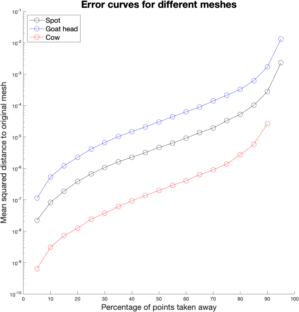
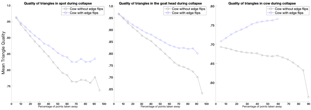
Another thing we measured was the quality of the mesh produced. Depending on the application, different measurements can be done. In our case, we have followed Liu et al. 2020 [7], which uses the quality measure \(Q_{ijk}\) defined in Section V.1. We average \(Q_{ijk}\) over all triangles in a mesh and plot the results across the percentage of vertices removed by edge collapses. Figure 10 shows the results for three different models.
Figure 10: variation of mean average quality along the hierarchy of meshes for three different models.
After the removal of approximately \(65 \%\) of the initial number of vertices, we notice that all meshes begin to level out and there is even marginal improvement for Spot the Cow model. Furthermore, we observe that the implementation of edge flips significantly increases the quality of the meshes produced. Unfortunately, we weren’t able to exploit its full capacity due to a lack of time and a bug in the code.
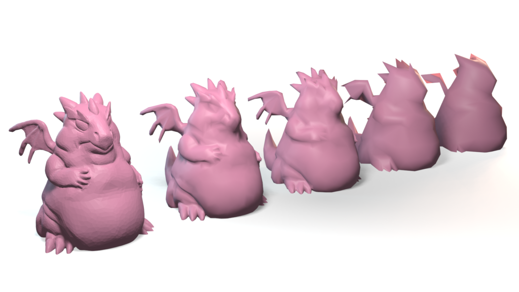
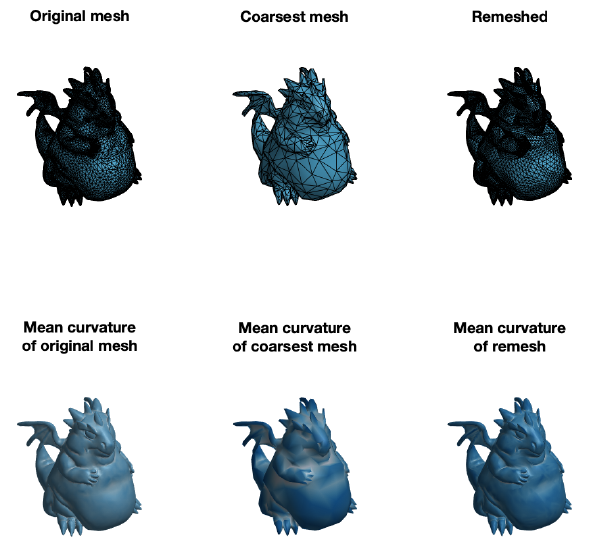
Finally, we have applied the self parameterization to perform remeshing. We have built a bijection \(\mathcal{M}^0\overset{f}{\longrightarrow}\mathcal{M}^L\) where \(\mathcal{M}^0\) is the coarsest mesh and \(\mathcal{M}^L\) is the original mesh. To remesh, we first upsample the topology of the coarse mesh \(M^{0}\), which adds more vertices and faces to the mesh. Subsequently, we use the bijective map to find correspondences between the upsampled mesh and the original mesh. With this correspondence, we build a new mesh with vertices lying inside the original. Figure 11 shows the result of the simplification followed by the remeshing process.
Figure 11: result of applying successive self-parameterization for remeshing. Given an initial fine mesh (left), it is simplified to a target number of faces (center). Then, this coarsest mesh is remeshed to match the original fine mesh (right). In the bottom row we can see the effect that this application has on the mean curvature.
VII. Conclusions and Future Work
In this project we explored hierarchical surface representations combined with successive self-parameterization, using mesh simplification to build a hierarchy of meshes and successive conformal mappings to build correspondences between different levels of the hierarchy. This allows to represent a surface with distinct levels of detail depending on the application. We investigated the application of the successive self-parameterization for remeshing and evaluated various quality metrics on the hierarchy of meshes, which provides meaningful insight into the preservation and loss of geometric data caused by the simplification process.
As main lines of future work, we envision using the successive self-parameterization to solve Poisson equations on curved surfaces, as done by Liu et al. 2021 [8]. While not yet complete, we started the implementation of the intrinsic prolongation operator, which is required for the geometric multigrid method to transfer solutions from coarse to fine meshes. Another step in this project could be creating a texture mapping between the course and fine mesh. Finally, another direction could be remeshing according to the technique using wavelets described in Khodakovsky et al. 2000 [1]. In this paper, wavelets are used to represent the difference between the coarsest and finest levels of a mesh.
While working on the application of Remeshing, that is, using the coarse mesh with upsampling and using the local information stored to reconstruct the geometry, we found that the edge flips after each collapse to be very promising. Based on that, we believe a more robust implementation of this idea can give better results in general. Moreover, we can use other remeshing operations when necessary. For example, tangential relaxation, edge splits and other operations might be useful for getting better-quality triangles. We have to be careful about how and when to apply edge splits, as applying them in each iteration would slow down the collapse convergence.
Another important line of work would be to improve performance and memory consumption in our implementation. While many operations were fully vectorized, there are still areas that can be improved.
We want to thank Professor Paul Kry for the guidance and mentorship (and patience on MATLAB debugging sessions) during these weeks. It is incredible how much can be learned and achieved in a short period of time with an enthusiastic mentor. We also want to thank the volunteers Leticia Mattos Da Silva and Erik Amézquita for all the tips and help they provided. Finally, we would like to thank Professor Justin Solomon for organizing SGI and making it possible to have a fantastic project with students and mentors from all over the world.
VIII. References
[1] Khodakovsky, A., Schröder, P., & Sweldens, W. (2000, July). Progressive geometry compression. In Proceedings of the 27th annual conference on Computer graphics and interactive techniques (pp. 271-278).
[2] Lee, A. W., Sweldens, W., Schröder, P., Cowsar, L., & Dobkin, D. (1998, July). MAPS: Multiresolution adaptive parameterization of surfaces. In Proceedings of the 25th annual conference on Computer graphics and interactive techniques (pp. 95-104).
[3] Mullen, P., Tong, Y., Alliez, P., & Desbrun, M. (2008, July). Spectral conformal parameterization. In Computer Graphics Forum (Vol. 27, No. 5, pp. 1487-1494). Oxford, UK: Blackwell Publishing Ltd.
[4] Lévy, Bruno, et al. “Least squares conformal maps for automatic texture atlas generation.” ACM transactions on graphics (TOG) 21.3 (2002): 362-371.
[5] Hoppe, H., DeRose, T., Duchamp, T., McDonald, J., & Stuetzle, W. (1993, September). Mesh optimization. In Proceedings of the 20th annual conference on Computer graphics and interactive techniques (pp. 19-26)
[6] Garland, M., & Heckbert, P. S. (1997, August). Surface simplification using quadric error metrics. In Proceedings of the 24th annual conference on Computer graphics and interactive techniques (pp. 209-216).
[7] Liu, H., Kim, V., Chaudhuri, S., Aigerman, N. & Jacobson, A. Neural Subdivision. ACM Trans. Graph.. 39 (2020)
[8] Liu, H., Zhang, J., Ben-Chen, M. & Jacobson, A. Surface Multigrid via Intrinsic Prolongation. ACM Trans. Graph.. 40 (2021)
[9] Levoy, M., Pulli, K., Curless, B., Rusinkiewicz, S., Koller, D., Pereira, L., Ginzton, M., Anderson, S., Davis, J., Ginsberg, J. & Others The digital Michelangelo project: 3D scanning of large statues. Proceedings Of The 27th Annual Conference On Computer Graphics And Interactive Techniques. pp. 131-144 (2000)
[10] Hormann, K., Lévy, B. & Sheffer, A. Mesh parameterization: Theory and practice. (2007)
[11] Li, W., Ray, N. & Lévy, B. Automatic and interactive mesh to T-spline conversion. 4th Eurographics Symposium On Geometry Processing-SGP 2006. (2006)
[12] Konaković, M., Crane, K., Deng, B., Bouaziz, S., Piker, D. & Pauly, M. Beyond developable: computational design and fabrication with auxetic materials. ACM Transactions On Graphics (TOG). 35, 1-11 (2016)
[13] Desbrun, M., Meyer, M. & Alliez, P. Intrinsic parameterizations of surface meshes. Computer Graphics Forum. 21, 209-218 (2002)
Latent NeRF (Neural Radiance Fields) is a state-of-the-art generative model capable of synthesizing 3D-consistent 2D images from a combination of 3D-sketch and text guides. In this report, we investigate the temporal consistency of Latent NeRF by generating 3D-consistent images with different sketch guides and exploring the interplay between 3D-sketch guidance and text prompts in the generation process; with a broader motivation of using diffusion models in animation and dynamic scene generation. Through our experiments, we discover the importance of incorporating both 3D sketch and text information to achieve accurate and consistent results. Additionally, we propose potential enhancements, including the integration of geometry/shape loss and automatic generation of descriptive text from geometry, to improve the model’s performance.
Introduction:
Neural Radiance Field (NeRF) is a relatively new representation of geometry. They use a neural network to approximate a function F: (x, θ) → (c, σ) that can model the appearance of a single scene. This function takes a sampled input 3D point x and a viewing direction θ derived from a 2D image (with camera information) and returns the color c = (r, g, b) and volume density σ of the shape at that point. This is enough to encode the shape and color of a scene as well as view-dependent lighting effects in the scene with a radiance field.
Traditionally, NeRFs have been trained with sets of images from the real world or images that are rendered using computer graphics software. Recently, image diffusion models such as Stable Diffusion have been able to generate coherent images from just text prompts. Combining diffusion models and NeRFs has led to Latent NeRF, a cutting-edge generative model that uses an image diffusion model to train NeRFs using just a text prompt and an optional guiding 3D shape.
We investigate the use of latent-nerf to create sequential images and animation. One major challenge in doing so is temporal consistency. It is currently challenging to ensure that diffusion models recreate the same object/character between runs. This week, we attempt to achieve temporal consistency of the model’s output and the influence of combining different input modalities.
Methodology:
We conducted a series of experiments to evaluate the temporal consistency of the Latent NeRF model and explore the interaction between sketches and text prompts during image synthesis.
Temporal Consistency Assessment:
We first decided to test consistency between two poses under the most naive approach to get a baseline for consistency in latent-nerf. We started by using sketch shapes to guide the shape of the NeRFs. Each sketch shape is a collection of simple triangle meshes arranged in roughly the same shape as the desired output. Our Blender-master of the team, Erik, created sketch shapes of a teddy bear in different poses and configurations to guide the NeRF generation. Figure 1 depicts the original sketch-shape of a teddy bear with its left arm raised, and Figure 2 shows the same teddy bear sketch with both arms down. Given the same text prompt, would the NeRFs generated from these sketch shapes look like the same object in different poses? According to the results in Figure 4 and Figure 5, the answer is no. The models have different colors, making them unsuitable to use as frames of animation.
Figure 1: Default teddy bear sketch with left arm up
Figure 2: Teddy bear sketch with both arms down
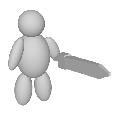
Figure 3: Teddy bear sketch holding a sword
Figure 4: Teddy with right arm up (default in Figure 1) sketch with the text prompt ‘a lego man’
Figure 5: Teddy with both hands down sketch (Figure 2) with the text prompt ‘a lego man’
Cross-Modal Interaction:
To understand the interplay between sketches and text prompts, we augmented the base sketch with a sword (Figure 3). We experimented with two different text prompts: “a lego man” (since this is the convention in previous papers to call it a “lego man” instead of a “lego human”) and “a lego man holding a sword”. Figure 6 illustrates the output when using the “a lego man” text prompt, which resulted in only the phantom of the sword being generated. However, when using the “a lego man holding a sword” text prompt, the model successfully generated a visible sword (Figure 7). The presence of both image and text prompts is crucial for generating visible new objects, suggesting the importance of cross-modal interaction.
Figure 6: Teddy holding a sword sketch with the text prompt ‘a lego man’
Figure 7: Teddy holding a sword sketch with the text prompt ‘a lego man holding a sword’
Additionally, we wanted to assess the level of support required from sketch-guidance while using text-guidance. To test this, we generated various lego humans based on specific instructions, such as ‘a lego man with right arm up’, ‘a lego man with left arm up’, while keeping the sketch guidance consistent with the same teddy sketch in Figure 1. As seen in Figures 8 and 9, despite the text prompts requesting opposite actions, the outputs are quite similar to each other, suggesting that text-guidance itself is not sufficient to generate the desired output.
Figure 8 : Default teddy sketch (Fig. 1) with the text prompt ‘a lego man with right arm up’
Figure 9: Default teddy sketch (Fig. 1) with the text prompt ‘a lego man with left arm up’
Discussion:
Our observations indicate that Latent NeRF’s temporal consistency can be improved by incorporating additional constraints and interactions between different input modalities. This suggests that using a long description of the desired character could enforce temporal consistency between poses.
Ideas:
Building on our observations and discussions, we have some ideas as to how to improve temporal consistency in Latent-NeRF. We could integrate a geometry/shape loss to enhance the model’s ability to maintain consistency between generated images. Additionally, we could develop a mechanism to automatically extract descriptive word descriptors from geometry to use as complementary text prompts. Finally, we could use Stable Diffusion concepts to guide consistency.
Potential Experiments:
Moving forward, we would like to explore the consistency in generating objects with similar geometry (e.g., different keywords as, sword, stick, etc. with the same sketch). To that end, we plan to repeat the same experiment, but with different combinations of geometry and text. Additionally, we would like to investigate the model’s performance when utilizing text prompts unrelated to the geometry, such as “stick” or “apple,” (when the sketch, in fact, displays a sword) to evaluate the robustness of cross-modal interactions. Lastly, we think it would be interesting to find/create a Stable Diffusion concept and apply it to the generation of two different poses.
Conclusion:
Our exploration of Latent NeRF’s temporal consistency and cross-modal interactions highlights the importance of combining sketch and text guides to achieve consistent and accurate 3D image synthesis. By addressing the observed issues and implementing potential enhancements, the model can be further refined to generate even more realistic and consistent images across different inputs. Eventually, this will help animators, modelers, and content creators to easily generate dynamic NeRFs with articulated characters and scenes.
Technical Journey:
Neural networks are renowned for their substantial computational demands, leading to extended training and inference times. Despite notable advancements in the realm of NeRFs research, which have contributed to improved training and inference speeds, these models continue to exhibit high memory requirements. Similarly, diffusion models also exhibit a pronounced appetite for memory resources. Consequently, the execution of Latent-NeRF necessitates access to machines equipped with GPUs boasting a minimum of 12 GB of VRAM.
The training of a single NeRF entails a substantial time investment, ranging from 30 minutes when using NVIDIA RX 3090 to 3 hours using Google Colab. Moreover, the implementation of latent NeRF entailed the integration of numerous dependencies, a process that demanded considerable troubleshooting efforts to ensure proper installation. Given the convergence of the two distinct areas of graphics research, namely NeRFs and Diffusion models, encountering technical challenges during dependency management was a foreseeable aspect of the endeavor. Such technical trouble shooting constitutes an inevitable and crucial facet of the overall research process.
Fortunately, the mentors of this project Sainan Liu, Ilke Demir and Olga Guțan, provided valuable guidance in navigating these technical complexities, which significantly expedited the resolution of issues and allowed us to focus more efficiently on the core aspects of our project.
Papers:
For temporal consistency with better texture/geometry details we explored: D-nerf, EditableNeRF, Tetra NeRF, NeRFEditing, One-2-3-45. For gometric manipulation for temporal consistent 3D animation generation with text/image guidance, SKED and DASR were reviewed.